1. Econometrics for Spatial RD Design

What's unique about Spatial RD

Forcing variable: two-dimensional vector (i.e. coordinates)

Cutoff: boundary lines

$\Rightarrow$ How should we extend the standard RD design?

Spatial RD specification

\begin{align*} y_{i} = \beta T_{i} + \gamma Dist_i + \delta T_{i} Dist_i + \mu_s + \varepsilon_{i} \end{align*}

Project coordinates into distance to boundary ($Dist_i$)

• $Dist_i < 0$ for control areas

Spatial RD specification (cont.)

\begin{align*} y_{i} = \beta T_{i} + \gamma Dist_i + \delta T_{i} Dist_i + \mu_s + \varepsilon_{i} \end{align*}

Then use standard RD design w/ boundary segment FE ($\mu_s$)

• $s$: segment that contains $i$'s nearest point on boundary

Why boundary segment fixed effects?

Without it, you would compare point $i$ to $k$ in diagram below

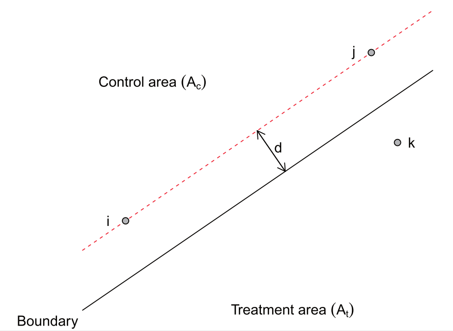
(Figure 3 of Keele & Titiunik 2014)

Threats to identification

Treatment boundary tends to overlap with other boundaries

e.g. School districts & media markets in U.S.

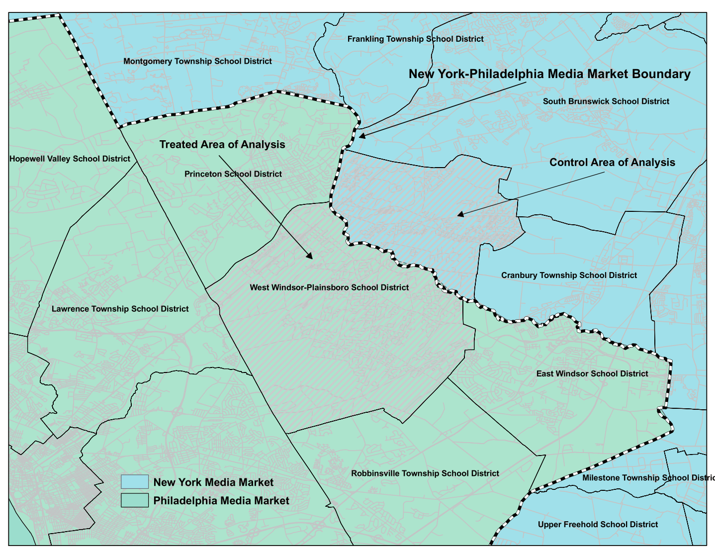(Figure 5 of Keele & Titiunik 2015)

$\Rightarrow$ Focus on segments where nothing else overlaps

Spatial RD example #1

Michalopoulos & Papaioannou (2014)

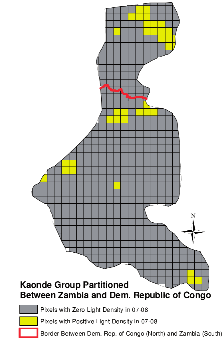
Ntnl govt quality $\Rightarrow$ development?

Look at ethnic homelands split by national boarders in Africa

• Segment FE = Ethnicity FE

Find no difference in nighttime light across border on average

Large heterogeneity across ethnic groups, though

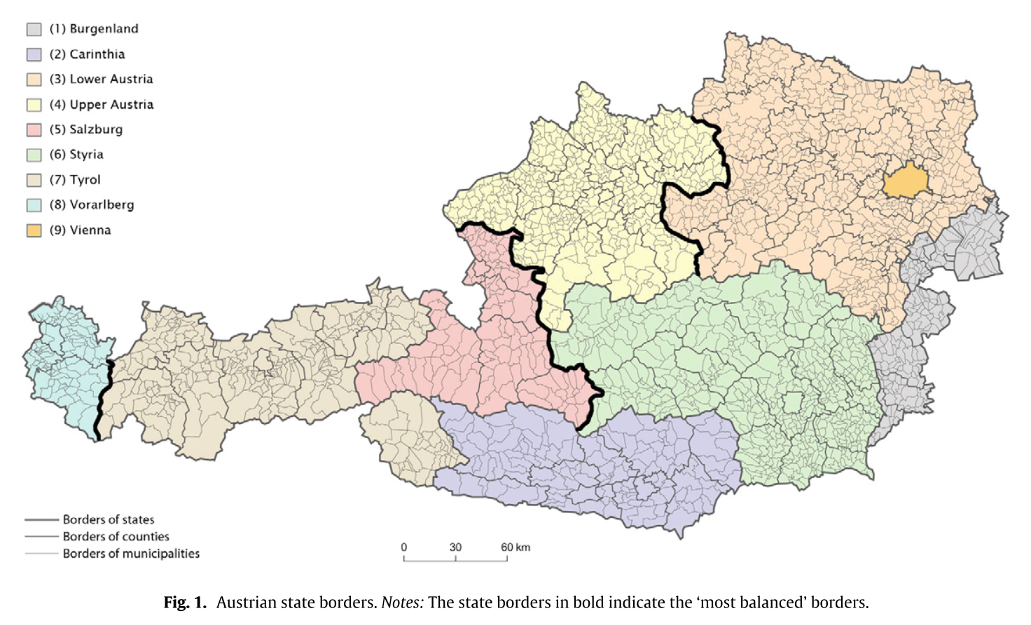
Spatial RD example #2

Berger et al. (2016)

Does higher TV license fees increase evasion in Austria?

Exploit differences in fees across states

Focus on state borders where covariates are balanced

2. Dell (2010)

Research question

Does forced labor system during Spanish colonial rule affect todya's living standards in Peru? If so, why?

Interesting?

• Yes, if why question is answered
• Lots of "history matters" papers already out there

Original?

• Focus on mechanism of long-run effect of history
• Pioneer in spatial RD design
• Findings go against well-known Engerman-Sokoloff hypothesis

Mita

1573-1812: Spanish colonial rule forced 1/7 of adult male population in parts of Peru & Bolivia to work in the Potosi silver & Huancavelica mercury mines

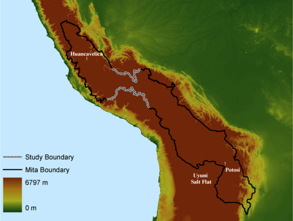
Communities subject to mita: clearly defined geographically

$\Rightarrow$ Spatial RD

Data for outcomes

Household consumption in 2001

Heights of 6-9 years old students

Road lengths by districts

• We will learn how to calculate this with elevation taken into consideration

Data for intermediate outcomes

% rural population in "hacienda" in 1689, 1845, 1940

• hacienda: large land-holding

Education in 1876, 1940, 2001

$\Rightarrow$ Allows to identify mechanisms

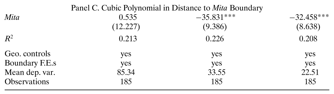
Results

Mita areas: worse-off today

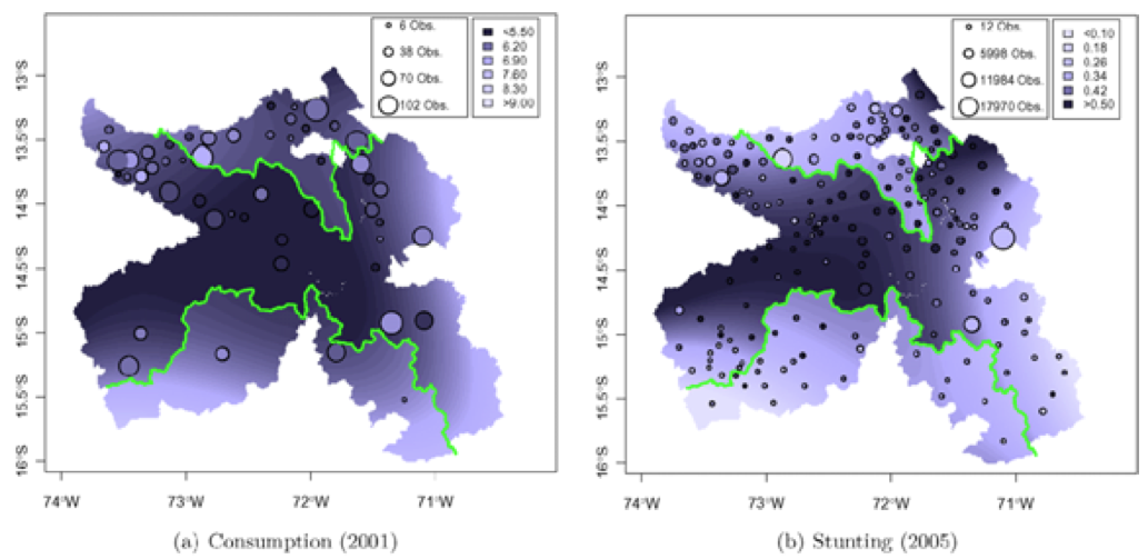
Figure 2 of Dell (2010)

Results (cont.)

Mita areas: worse-off today

Historically, less educated & more equal in land holding

$\Rightarrow$ Against the Engerman-Sokoloff hypothesis (see Sokoloff & Engerman 2000)

Prepare for the rest of this lecture

1. Launch ArcMap 10 (it takes time)

2. Download the zipped dataset for Lecture 7

3. Save it to Desktop (C:\\Users\\yourname\\Desktop)

• Don't save in the remote server, which slows down ArcGIS

4. Right-click it and choose 7-Zip > Extract to "Lecture7\"

• So the directory path will be: C:\\Users\\yourname\\Desktop\\Lecture7

Prepare for the rest of this lecture (cont.)

Now in ArcMap's Catalogue Window:

5. Establish connection to data folder

• Right-click Folder Connections
• Select Connect to Folder
• Choose Desktop > Lecture7

6. Right-click input/w100s10.***.zip and select 7-Zip > Extract Here

• These four files are SRTM30 data for the area around Peru (cf. Lecture 6)

Prepare for the rest of this lecture (cont.)

7. Prepare the Model Builder

• Create a Model
• Save it as code/models.tbx/exercises1-3
• Repeat for another model called exercise4

Coordinate system for Lecture 7 data

Now browse data in the input/ folder

What coordinate system do they use? (cf. Lecture 1)

Coordinate system for Lecture 7 data (cont.)

It's UTM Zone 18S (cf. Lecture 3)

$\Rightarrow$ Calculation of surface area and distance is straightforward

Always pay attention to the coordinate system of the spatial data you use

3. Geo-processing for Spatial RD Design

Spatial RD Design Data Generation

\begin{align*} y_{i} = \beta T_{i} + \gamma Dist_i + \delta T_{i} Dist_i + \mu_s + \varepsilon_{i} \end{align*}

1. Treatment indicator ($T_i$)

2. Treatment boundary polylines

3. Boundary segment indicator ($\mu_s$)

4. Distance to boundary ($Dist_i$)

Exercise #1

Attach mita district indicator

Inputs:

1. District polygons (StudyDistricts.shp)

• District ID: dist_id

2. List of mita districts (districts.txt)

• District ID: dist_id
• Mita indicator: mita

Exercise #1 (cont.)

Geo-processing tools to be used for this exercise:

1. Table to Table

• Convert the table in text format into dBASE
• Otherwise Join Field does not work

2. Copy Features + Join Field

• Attach mita indicator to district polygons
• cf. Lecture 6 Exercise 4 Step 1

Exercise #1: Step 1

Table to Table

Input Rows: ...\Lecture7\input\districts.txt

Output Location: ...\Lecture7\temporary

• Directory in which the output table is saved

Output Table: districts.dbf

Expression: leave it blank

• Can be used to keep only some rows

Field Map: leave as it is

Exercise #1: Step 2

Copy Features

Input Features: ...\Lecture7\input\StudyDistricts.shp

Output Feature Class: ...\Lecture7\temporary\mita_districts.shp

• Do not name the output as districts.shp
• Its attribute table will then have the same file name as the output from Table to Table

Exercise #1: Step 2

Join Field

Input Table: mita_districts.shp

• Output from Copy Features

Input Join Field: dist_id

Join Table: districts.dbf

• Output from Table To Table

Output Join Field: dist_id

Join Fields: mita

Exercise #1 (cont.)

Now save and run the Model.

Browse the attribute table of the output

Is everything as expected?

Exercise #2

Mita boundary polyline

Geoprocessing tools:

1. Dissolve

• Create mita area polygon and non-mita area polygon

2. Polygon To Line + Select

• Convert polygons to their boundary polylines
• Then keep those tangent on the other polygons

Polygon To Line

(Image taken from ArcGIS Help on Polygon To Line)

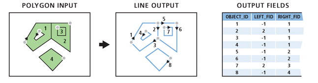
For treatment boundary polylines

$\Rightarrow$ LEFT_FID $\neq$ -1

Exercise #2: Step 1

Dissolve

Input Features: mita_districts.shp (2)

• Output from Join Field

Output Feature Class: ...\Lecture7\temporary\mita_area.shp

Dissolve_Field(s): mita

Check "Create multipart features"

Now run the model and see how the output looks like

Exercise #2: Step 2

Polygon To Line

Input Features: mita_area.shp

• Output from Dissolve

Output Feature Class: ...\Lecture7\temporary\polygon2line.shp

Check "Identify and store polygon neighboring information"

• If unchecked, each polygon becomes one polyline

Now run the model and see how the output looks like

Exercise #2: Step 3

Select

Input Features: polygon2line.shp

• Output from Polyline To Line

Output Feature Class: ...\Lecture7\temporary\boundary.shp

Expression: "LEFT_FID" <> -1

• Enclose field name with " "
• <> means not equal to

Now run the model and see how the output looks like

Exercise #2 (cont.)

Alternative solution

1. Select with "mita" = 1

• Create a mita area polygon

2. Select with "mita" = 0

• Create a non-mita area polygon

3. Intersect with output type LINE

• Intersection of the two polygons will be kept as a polyline
• With output type INPUT, no feature will be created

Distance to boundary

Can now be calculated by Near tool with the boundary polyline as near feature

• cf. Lecture 4 Exercise 1 Step 2

But we also need "boundary segment fixed effects that denote which of four equal length segments of the boundary is the closest to the observation’s district capital" (Dell 2010, p. 1870)

$\Rightarrow$ Split each boundary line by half

Exercise #3: Overview

Bounday segment fixed effects

Geo-processing tools:

1. Unsplit Line

• Convert each boundary into one polyline
• Necessary because Polygon To Line fails to create one polyline for the southern boundary...

2. Add Field + Calculate Field (cf. Lecture 5)

• Add midpoint coordinates

Exercise #3: Overview (cont.)

3. Make XY Event Layer + Copy Features

• Create midpoint point features

4. Split Line at Point

• Divide each boundary at midpoint

5. Copy Features + Near (w/ district capitals as input)

• Attach boundary segment indicator
• Calculate distance to boundary

Exercise #3: Step 1

Unsplit Line

Input Features: boundary.shp

• Output from Select

Output Feature Class: ...\Lecture7\temporary\boundary_unsplit.shp

Now run the model and see how the output looks like

Exercise #3: Step 2

Midpoint coordinates

We will add two new fields

• One for midpoint longitude
• The other for midpoint latitude

$\Rightarrow$ Use Add Field + Calculate Field twice

Exercise #3: Step 2 (cont.)

Add Field

Input Table: boundary_unsplit.shp

Field Name: midpoint_X / midpoint_Y

• Or whatever you prefer (not exceeding 10 characters)

Field Type: DOUBLE

• We want to have the exact coordinate

Exercise #3: Step 2 (cont.)

Calculate Field

Input Table: boundary_unsplit.shp

• Output from Add Field

Field Name: midpoint_X / midpoint_Y

• Or the same as what you specified in Add Field

Expression: see next slide

Expression Type: PYTHON_9.3

position Along Line method

For midpoint_X:

!shape!.positionAlongLine(0.5,True).firstPoint.X

For midpoint_Y:

!shape!.positionAlongLine(0.5,True).firstPoint.Y

position Along Line method

For midpoint_X:

!shape!.positionAlongLine(0.5,True).firstPoint.X

For midpoint_Y:

!shape!.positionAlongLine(0.5,True).firstPoint.Y

0.5 for mid points

• Change this fraction for other points on polyline

• For multiple points, we can use loop over values in Python (cf. Lecture 6)

An alternative for calculating midpoint coordinates

Use the Add Geometry Attributes tool

• For Geometry Properties, choose LINE_START_MID_END
• Then use the fields named MID_X and MID_Y for next step

Exercise #3: Step 3

Make XY Event Layer

XY Table: boundary_unsplit.shp (5)

• Output from Calculate Field (2)

X Field: midpoint_X

Y Field: midpoint_Y

Spatial Reference: WGS_1984_UTM_Zone_18S

• Make sure using the same coordinate system as boundary polylines

Exercise #3: Step 3 (cont.)

Copy Features

Input Features: output from Make XY Event Layer

Output Feature Class: ...\Lecture7\temporary\midpoints.shp

Now run the model and see how the output looks like

Exercise #3: Step 4

Split Line at Point

Input Features: boundary_unsplit.shp (5)

• Output from Calculate Field (2)

Point Features: midpoints.shp

• Output from Copy Features (2)

Output Feature Class: ...\Lecture7\output\boundary_segments.shp

Now run the model and see how the output looks like

We're now ready to calculate the distance to the boundary

Exercise #3: Step 5

Copy Features

• To avoid overwriting the original file by Near tool

Input Features: ...\Lecture7\input\district_capitals.shp

Output Feature Class: ...\Lecture7\temporary\distance2border.shp

Exercise #3: Step 5 (cont.)

Near

Input Features: distance2border.shp

Near Features: boundary_segments.shp

Check "Location"

• We don't need this, but can be used for error checking

Method: PLANAR

• Because we're using UTM projection, not WGS 1984

Exercise #3 (cont.)

Now save and run the Model.

Browse the output attribute table.

NEAR_FID: Nearest boundary segment ID

• Same as FID in boundary_segments.shp

NEAR_DIST: Distance to boundary (in meters)

Finally, use Table to Excel to export an Excel sheet (we skip this today)

Solutions for Excercises 1-3

Look at

• lec7models.tbx\exercises1-3
• exercises1-3.py

in the solutions4exercises\ folder

For the Python script, you have to edit arguments for:

• Table To Table
• Join Field
• Near

so that all the file paths are relative.

4. Calculate 3D polyline length

Road length in hilly areas

Peru is a hilly country

$\Rightarrow$ Ignoring elevation can be misleading

$\Rightarrow$ Use the Add Surface Information tool

Add Surface Information

Take elevation raster and vector data as inputs

Add new fields to the input attribute table (i.e. overwriting)

• 3D length for polylines
• 3D surface area for polygons

For more detail, see ArcGIS Help

Add Surface Information (cont.)

This tool is part of 3D Analyst extension

Click "Tool > Extensions" to activate the extension in ArcMap

In Python, add the following command line:

arcpy.CheckOutExtension("3D")

Exercise #4: Overview

Road length by district

Inputs:

Road polylines for Peru (roads_prj.shp)

• Coordinate system: UTM 18S

STRM30 (W100S10.DEM)

• Coordinate system: WGS 1984

Exercise #4: Overview (cont.)

Geo-processing tools:

1. Select

• for obtaining length by road type

2. Intersect + Dissolve

• for obtaining total length by district

3. Project Raster

• Polyline length calculation requires UTM projection

4. Add Surface Information

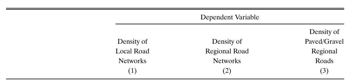
Codebook for road data

(according to maketable8.do in the Dell (2010) replication files)

RUTA: type of road

• Departamental: Regional
• Vecinal: Local

SUPERFICIE: road condition

1. Paved
2. Gravel
3. non-gravel
4. trocha carrozable (?)
5. Under construction
9. Planned

Dell (2010) Table VIII

Exercise #4: Step 1

Select

Input Features: ...\Lecture7\input\roads_prj.shp

Output Feature Class: ...\Lecture7\temporary\roads_paved.shp

Expression:

"RUTA" = 'Departamental' AND ("SUPERFICIE" = 1 OR "SUPERFICIE" =2)

• Field name: enclosed by ""
• String value: enclosed by ''
• AND / OR: logical operator

Exercise #4: Step 1 (cont.)

For regional roads:

"RUTA" = 'Departamental' AND "SUPERFICIE" >= 1 AND "SUPERFICIE" <=4

For local roads:

"RUTA" = 'Vecinal' AND "SUPERFICIE" >= 1 AND "SUPERFICIE" <=4

Now run the model and see how the output looks like

Exercise #4: Step 2

Intersect

Input Features:

• roads_paved.shp
• ...\input\StudyDistricts.shp

Output Feature Class: ...\temporary\intersect_paved.shp

Output Type: INPUT

Exercise #4: Step 2 (cont.)

Dissolve

Input Features: intersect_paved.shp

Output Feature Class: ...\temporary\district_road_paved.shp

Dissolve_Field(s): dist_id

Check "multipart features"

Now run the model and see how the output looks like

Projecting raster data

Now we need to project elevation data to UTM

Which involves resampling (i.e. interpolation)

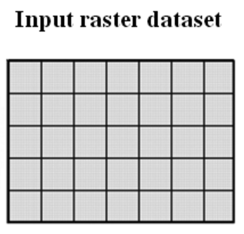
	$\Rightarrow$
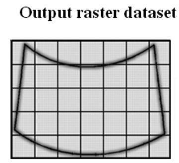
Raster in WGS 1984		Raster in UTM

Cell in WGS1984 $\neq$ Cell in UTM

(image source)

Exercise #4: Step 3

Project Raster

Input Raster: ...\input\W100S10.DEM

Output Feature Class: ...\temporary\elevation_prj.tif

Output Coordinate System: WGS_1984_UTM_Zone_18S

Resampling Technique: Bilinear or Cubic

• NEAREST or MAJORITY: for categorical raster

Output Cell Size: 1000 for X / 1000 for Y

• 30 arc-sec $\approx$ 1km
• Default value can also be used

Exercise #4: Step 4

Add Surface Information

Input Feature Class: district_road_paved.shp

• Output from Dissolve

Input Surface: elevation_prj.tif

• Output from Project Raster

Output Property: SURFACE_LENGTH

NOTE: This tool overwrites the input data.

Exercise #4: Step 5

Table To Excel

Input Table: district_road_paved.shp (2)

• Output from Add Surface Information

Output Excel File: ...\output\district_road_paved.xls

Loop over road types in Python

We need to repeat

• Select
• Intersect
• Dissolve
• Add Surface Information
• Table To Excel

for each road type

We can use Python's list loop (cf. Lecture 6)

Loop over road types in Python (cont.)

1. Create the list of road type names

						
							road_types = ["paved","regional","local"]
						
					

2. Start the loop over road types

						
							for road_type in road_types:
						
					

Loop over road types in Python (cont.)

3. Change the output file names by string concatenation

						
road_types = ["paved","regional","local"]
for road_type in road_types:

  print "...Intermediate files being set"
  roads_shp = "temporary\\roads_"+road_type+".shp"
  intersect_shp = "temporary\\intersect_"+road_type+".shp"
  district_road_shp = "temporary\\district_road_"+road_type+".shp"

  print "...Output files being set"
  district_road_xls = "output\\district_road_"+road_type+".xls"

						
					

Loop over road types in Python (cont.)

4. For Select, use if/elif/else statements

						
if road_type == "paved":
  selection_criteria = "\"RUTA\" = 'Departamental' AND ( \"SUPERFICIE\" = 1 OR \"SUPERFICIE\" = 2 )"

elif road_type == "regional":
  selection_criteria = "\"RUTA\" = 'Departamental' AND ( \"SUPERFICIE\" >= 1 OR \"SUPERFICIE\" <= 4 )"

else:
  selection_criteria = "\"RUTA\" = 'Vecinal' AND ( \"SUPERFICIE\" >= 1 OR \"SUPERFICIE\" <= 4 )"

arcpy.Select_analysis(roads_prj_shp, roads_by_type_shp, selection_criteria)
						
					

"Model" model for Excercise 4

lec7models.tbx\exercise4

Model Python Script for Lecture 7

exercise4.py