Causal Inference with Spatial Data
(ArcGIS 10 for Economics Research)
Lecture 6
Elevation
Masayuki Kudamatsu
16 November, 2018
Press SPACE to proceed.
To go back to the previous slide, press SHIFT+SPACE.
Today's road map
1. Elevation in economics
2. Duflo & Pande (2007)
3. Replicate instruments in Duflo & Pande (2007)
4. Calculate polyline length
5. Loop over values in Python
1. Elevation in economics
It's a great source of exogenous variation!
Dinkelman (2011)
Electrification in South Africa (1996-2001)
$\Rightarrow$ Female labor supply $\uparrow$
Electrification: instrumented by mean land gradient
- Flat terrain: cheap to lay power lines
Qian (2008)
Tea production $\uparrow$ in China due to liberalization in 1979
$\Rightarrow$ Male-to-female ratio $\downarrow$
Tea production: instrumented by mean land gradient
- Tea grows in hilly terrain
Yanagizawa-Drott (2014)
Anti-Hutu radio station in Rwanda
$\Rightarrow$ Genocide incidents $\uparrow$
Radio: instrumented by signal strength
2. Duflo & Pande (2007)
Research Question
Do irrigation dams improve agricultural production and reduce rural poverty in India?
Important?
- Dams: built on nearly 1/2 of rivers worldwide
- Believed to reduce poverty, but no credible evidence
Original?
- Use geography to obtain credible impact estimates
Feasible?
Data
Unit of analysis: districts
Agricultural production data: annual 1971-99
Poverty data: 1973, 83, 87, 93, 99
Dams: location (nearest city), data of completion
- Source: World Registry of Large Dams
Identification strategy
Dam constriction: instrumented by river gradient
$\Leftarrow$ Dams: easier to build if river gradient is
- Moderate for irrigation dams
- Very steep for hydroelectricity dams
How to use time-invariant river gradient for panel regression?
1st stage
\begin{align*} D_{ist} =& \ \sum_{k=2}^4 \alpha_k (RGr_{ki} \ast \bar{D}_{st}) + (\mathbf{M}'_i \ast \bar{D}_{st})\boldsymbol{\beta} \\ & + \sum_{k=2}^4 \gamma_k (RGr_{ki} \ast l_{t}) + \nu_i + \mu_{st} + \omega_{ist} \end{align*}
| $D_{ist}$ | # dams in district $i$ state $s$ in year $t$ |
| $RGr_{ki}$ | Fraction of river areas in gradient category $k$ |
| (2 for 1.5-3%; 3 for 3-6%, 4 for over 6%) |
We will learn how to calculate $RGr_{ki}$ in ArcGIS
1st stage (cont.)
\begin{align*} D_{ist} =& \ \sum_{k=2}^4 \alpha_k (RGr_{ki} \ast \bar{D}_{st}) + (\mathbf{M}'_i \ast \bar{D}_{st})\boldsymbol{\beta} \\ & + \sum_{k=2}^4 \gamma_k (RGr_{ki} \ast l_{t}) + \nu_i + \mu_{st} + \omega_{ist} \end{align*}
| $\bar{D}_{st}$ | Predicted # of dams in state $s$ in year $t$ $=\frac{D_{s,1970}}{\sum_s D_{s,1970}}*\sum_s D_{st}$ ($D_{st}$: # dams in state $s$ in year $t$) |
| $\Leftarrow$ $D_{st}$ is endogenous to poverty |
Annual total # of dams in India ($\sum_s D_{st}$)
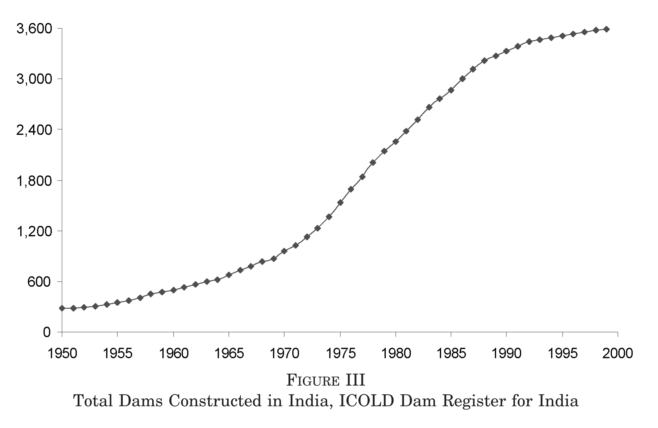
(Figure III of Duflo and Pande 2007)
1st stage (cont.)
\begin{align*} D_{ist} =& \ \sum_{k=2}^4 \alpha_k (RGr_{ki} \ast \bar{D}_{st}) + (\mathbf{M}'_i \ast \bar{D}_{st})\boldsymbol{\beta} \\ & + \sum_{k=2}^4 \gamma_k (RGr_{ki} \ast l_{t}) + \nu_i + \mu_{st} + \omega_{ist} \end{align*}
| $\mathbf{M}_i$ | Controls: river length, fraction of district areas with each gradient cateogry, etc. |
| $l_{t}$ | Year dummies |
| $\nu_i,\mu_{st}$ | District and state-year FEs |
Why should we control for each of these variables?
1st stage (cont.)
\begin{align*} D_{ist} =& \ \sum_{k=2}^4 \alpha_k (RGr_{ki} \ast \bar{D}_{st}) + (\mathbf{M}'_i \ast \bar{D}_{st})\boldsymbol{\beta} \\ & + \sum_{k=2}^4 \gamma_k (RGr_{ki} \ast l_{t}) + \nu_i + \mu_{st} + \omega_{ist} \end{align*}
| $\mathbf{M}_i$ | Controls: river length, fraction of district areas with each gradient cateogry, etc. |
| $l_{t}$ | Year dummies |
| $\nu_i,\mu_{st}$ | District and state-year FEs |
We will learn how to obtain river length in $\mathbf{M}_i$
2nd stage
\begin{align*} y_{ist} =& \ \gamma_i + \eta_{st} + \delta D_{ist} + \delta^U D_{ist}^U \\ & + \mathbf{Z}_{ist}\mathbf{\delta_Z} + \mathbf{Z^U}_{ist}\mathbf{\delta_Z^U} + \varepsilon_{ist} \end{align*}
| $y_{ist}$ | Agricultural outcomes / poverty measures |
| $D_{ist}$ | # of dams in own district (harmful) |
| $\Leftarrow$ Displacement, soil degradation, restricted water use | |
| $D_{ist}^U$ | # of dams in upstream districts (beneficial) |
| $\Leftarrow$ Irrigation | |
| $\mathbf{Z}_{ist}$ | All the controls for own district |
| $\mathbf{Z^U}_{ist}$ | All the controls for upstream districts |
2nd stage (cont.)
\begin{align*} y_{ist} =& \ \gamma_i + \eta_{st} + \delta D_{ist} + \delta^U D_{ist}^U \\ & + \mathbf{Z}_{ist}\mathbf{\delta_Z} + \mathbf{Z^U}_{ist}\mathbf{\delta_Z^U} + \varepsilon_{ist} \end{align*}
$D_{ist}$: instrumented by fitted value from 1st stage
$D_{ist}^U$: instrumented by sum of fitted values from 1st stage for upstream districts
cf. Using the fitted value from 1st stage as IV yields the 2SLS estimator (see Section 9.5.1 of Greene (2000), p. 374)
1st stage results
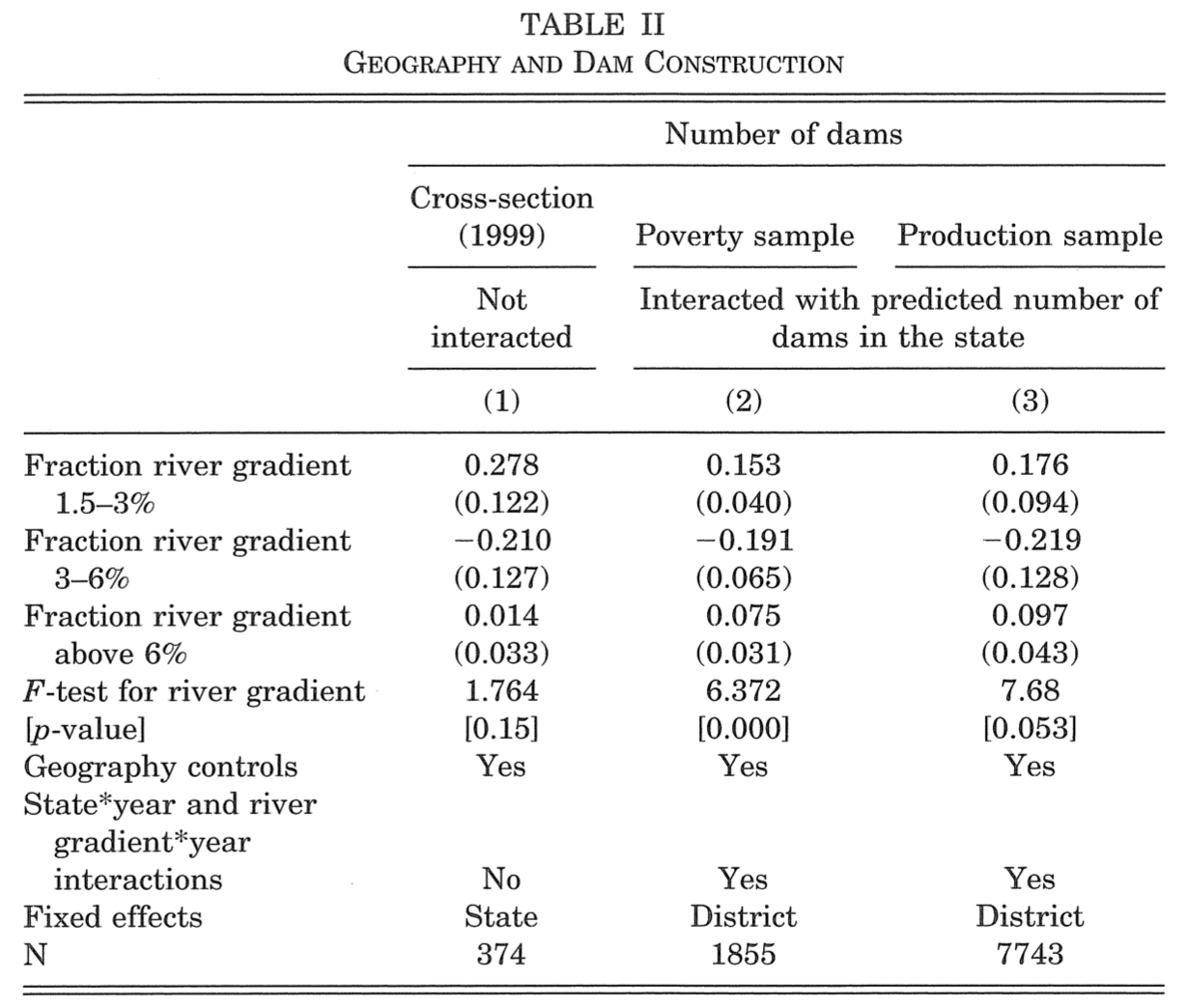
(Table II of Duflo and Pande 2007)
2nd stage results (on agriculture)
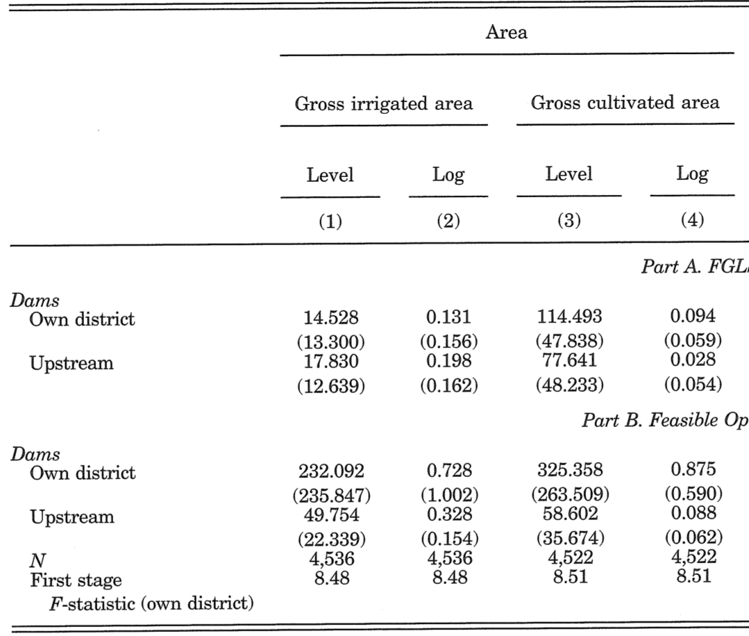
(Table III of Duflo and Pande 2007)
2nd stage results (on agriculture)
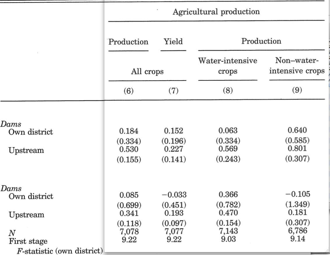
(Table III of Duflo and Pande 2007)
2nd stage results (on poverty)
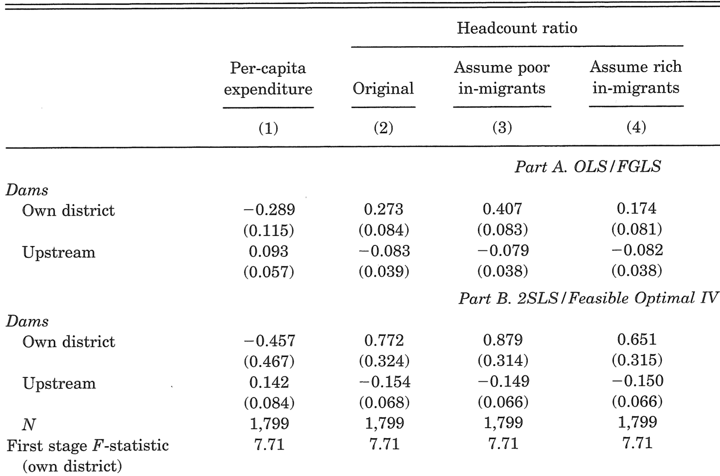
(Table VIII of Duflo and Pande 2007)
Prepare for the rest of this lecture
1. Launch ArcMap 10 (it takes time)
2. Download the zipped dataset for Lecture 6
3. Save it to Desktop (C:\\Users\\yourname\\Desktop)
4. Right-click it and choose 7-Zip > Extract to "Lecture6\"
-
So the directory path will be:
C:\\Users\\yourname\\Desktop\\Lecture6
In the input folder:
5. Right-click 10m-rivers-lake-centerlines.zip and select 7-Zip > Extract to Here
Prepare for the rest of this lecture (cont.)
Now in ArcMap's Catalogue Window:
6. Establish connection to data folder
- Right-click Folder Connections
- Select Connect to Folder
- Choose Desktop > Lecture6
7. Create two empty models in the code/models.tbx
-
exercises1-3 -
exercise4
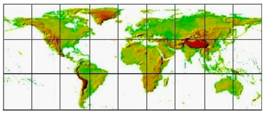
Elevation data
We use SRTM30 (version 2.1)
- It supersedes GTOPO30 used by Duflo and Pande (2007)
- WorldDEM is an updated version, but not for free of charge
Resolution: 30x30 arc seconds (roughly 1x1km)
Avaialable in 27 separate tiles
How to use SRTM30 in ArcGIS 10
1. Log on to: webgis.com/srtm30.html
2. Click the tile covering your study area
3. Download:
-
***.dem.zip(data file) -
***.hdr.zip(header file) -
***.prj.zip(projection file) -
***.stx.zip(statistics file)
For this lecture, these four files for India (060n40.***.zip) are already downloaded
in the input/ folder.
How to use SRTM30 in ArcGIS 10 (cont.)
4. Unzip them so the four files (.DEM, .HDR, .PRJ, .STX) are all saved in the same directory
- Right-click each .zip file and choose 7-Zip > Extract Here
5. Drag the .DEM file from ArcMap's Calatogue window
6. For geo-processing, use the .DEM file as the input file
7. If you use multiple tiles, Mosaic to New Raster appends them all
Mosaic to New Raster
Make sure to set the appropriate pixel type
-
By default, it sets
8_BIT_UNSIGNED(i.e. 0 to 255) - If your raster data is in decimals, negative values, or larger than 255, it gets distorted
-
For elevation data, choose
16_BIT_SIGNED(i.e. -32,768 to 32,767)
3. Replicate Instruments in Duflo & Pande (2007)
Data we want to construct
District-level data on fraction of river areas with gradient:
- 1.5-3%
- 3-6%
- 6% or steeper
$\Rightarrow$ Obtain gradient of each segment of river by matching river polylines with gradient raster:
Data we want to construct (cont.)
If each raster cell is not of equal size within a district
- Each cell is large
- The district stretches a lot along the north-south direction
$\Rightarrow$ Need to project the raster data (cf. Lecture 7)
Data we want to construct (cont.)
But this lecture assumes:
Each river segment is of equal size within the same district
- Districts in India are at most 3° wide in latitude
- India is located from 8° to 37° North
- 1° in longitude at 15° = 107.551km
- 1° in longitude at 30° = 96.486km
- 30 seconds in longitude can differ up to only 18m
$\frac{107551-96486}{120}*\frac{3}{30-15} \approx 18$
Data we want to construct (cont.)
If each river segment is of equal size,
$\Rightarrow$ We can use Zonal Statitics (cf. Lecture 5) with two inputs:
- River polylines
- Indicator raster for each gradient category
- 1 for (say) 3-6%
- 0 otherwise
| Mean cell value among river cells | = | Fraction of river areas with gradient 3-6% |
| $\uparrow$ | ||
| Zonal Statistics |
Data we want to construct (cont.)
1. Indicator raster for each gradient category
- 1.5-3%
- 3-6%
- 6% or steeper
2. River polylines intersected & dissolved by district
3. % of river segments in each gradient category
- Use Zonal Statistics with 1 and 2 as inputs
Exercise #1: Overview
Indicator raster for each gradient category
Input: elevation data (E060N40.DEM)
Geo-processing tools:
1. Slope
- Transform elevation to gradient
2. Reclassify (Spatial Analyst)
- Create indicator raster cells
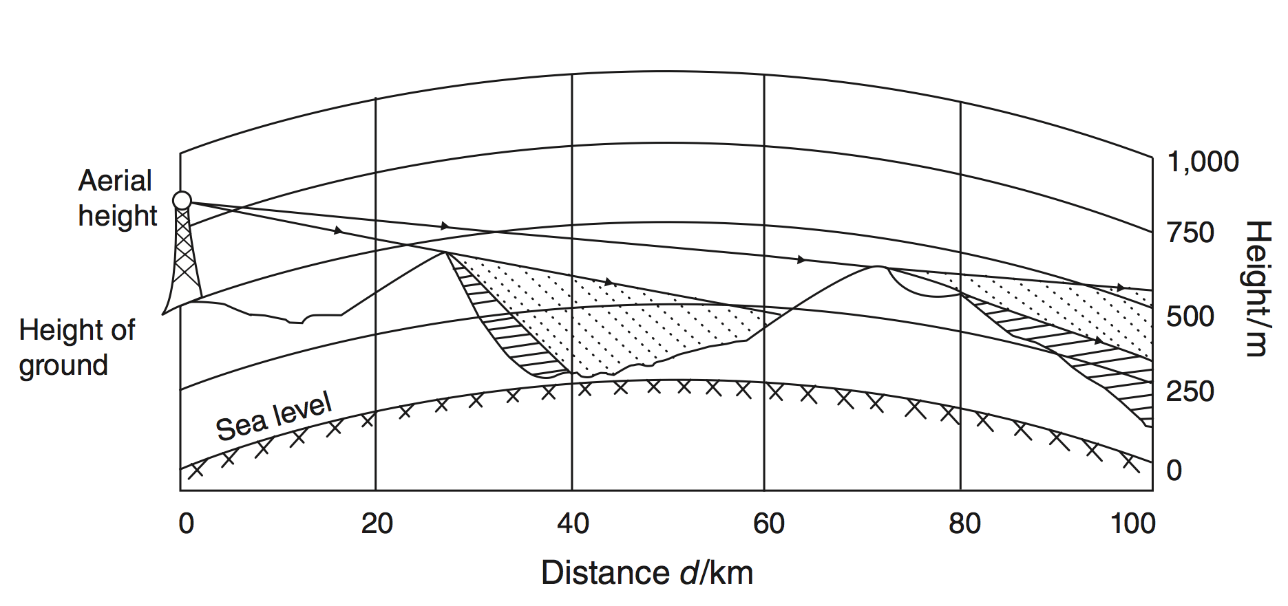
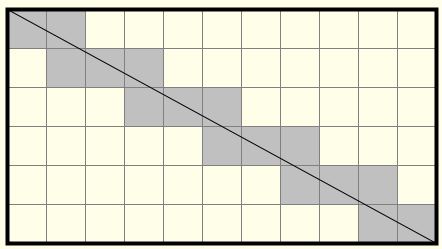
What Slope tool does
Return either $\theta$ or $\tan\theta$ in diagram below
What Slope tool does (cont.)
$\tan\theta$ for cell $e$ is obtained by
\begin{align*} \Rightarrow \ \tan \theta = \sqrt{(dz/dx)^2+(dz/dy)^2} \end{align*}
where
\begin{align*} \frac{dz}{dx} = & \ \Big[\frac{c + 2f + i}{4} - \frac{a+2d+g}{4}\Big] / 2 \\ \frac{dz}{dy} = & \ \Big[\frac{a+2b+c}{4} - \frac{g + 2h + i}{4}\Big] / 2 \end{align*}
Exercise #1: Step 1
SLOPE
Input raster: ...\Lecture6\input\E060N40.DEM
Output raster: ...\Lecture6\temporary\slope.tif
Output Measurement: PERCENT_RISE
- Duflo & Pande (2007) use gradient in % (i.e. $\tan\theta\times 100$)
- If you need $\theta$, choose DEGREE instead
Z factor: 0.000009
- # of (x,y) units in one z unit
- 0.000009° = 1m
Z-factor
1 if raster data is in projected coordinate system
- If coordinates and elevation are in different units (e.g., feet vs meters), use appropriate conversion factor
0.000009 if geographic coordinate system and low-latitude areas
- 1° $\approx$ 111,120 meters
For middle- to high-latitude areas, use Project Raster first to use UTM projections (cf. Lecture 7)
- 1° in longitude < 1° in latitude
Exercise #1: Step 2
RECLASSIFY
Input raster: slope.tif
- Output from Slope tool
Reclass field: VALUE
Reclassification: see next slide
Output raster: ...\Lecture6\temporary\gradient3060.tif
Uncheck "Change missing values to NoData"
RECLASSIFY (cont.)
For gradient 3-6%:
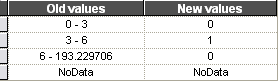
- Select rows other than NoData; then click "Delete Entries"
- Click "Add Entry"; then click each cell to enter values
- For a range of values, enter spaces before/after hyphen
- For max value, browse input raster (slope.tif) in ArcMap
- Use comma (,) for decimal marks if you live in one of these countries.
Exercise #1 Step 2 (cont.)
Repeat for gradient 1.5-3% and over 6%
Exercise #2: Overview
River polylines by district
Inputs:
Natural Earth 1:10m river + lake centerlines (ne_10m_river_lake_centerlines.shp)
- Digital Charts of the World, used by Duflo & Pande (2007), was made in 1992
- Natural Earth: updated alternative
Indian district polygons (gadm36_IND_2.shp)
- Provided by GADM
Exercise #2: Overview (cont.)
Geo-processing tools:
1. Intersect
- Cut rivers by district boundaries
2. Dissolve
- Turn all river polylines within a district into one feature
cf. Lecture 5
Exercise #2: Step 1
Intersect (Analysis)
Input Features (both in ...\Lecture6\input\):
gadm36_IND_2.shp
ne_10m_rivers_lake_centerlines.shp
- Click the directory icon to choose input data
- If the data is shown in ArcMap, it appears in the drop-down menu. But then the data file name won't properly be exported in a Python script.
Output Feature Class: ...\Lecture6\temporary\intersect.shp
Exercise #2: Step 2
Dissolve (Data Management)
Input Features: intersect.shp
- Output from Intersect
Output Feature Class: ...\output\river_by_district.shp
- We will use this data for Exercise #3
Dissolve_Field(s): GID_2
- Unique district ID
Check "Create multipart features"
Dissolve (Data Management) (cont.)
Statistics Field(s)
NAME_1 FIRST
NAME_2 FIRST
- To keep state and district names
- Choose FIRST (or LAST) for string fields
Exercise #2 (cont.)
Now save and run the Model.
Browse river_by_district.shp
To check if multipart features are properly created:
-
Browse
river_by_disrict.shpandgadm36_IND_2.shp - Select a district with multiple rivers by cursor
-
See attribute table of
gadm36_IND_2.shpfor GID_2 of the selected district -
See attribute table of
river_by_disrict.shpand select the row for this GID_2
Exercise #3
Fraction of river areas with each gradient category
Geo-processing tools:
1. Zonal Statistics as Table
2. Table To Excel
Exercise #3: Step 1
Zonal Statistics as Table
Input raster or feature zone data: river_by_district.shp
- Output from Dissolve
Zone field: GID_2
Input value raster: gradient3060.tif
- Output from Reclassify
Output Table: ...\temporary\river_gradient3060.dbf
Check "Ignore NoData in calculation"
Statistics type: MEAN
Exercise #3 Step 2
Table To Excel
Input Table: river_gradient3060.dbf
Output Excel File: ...\Lecture6\output\river_gradient3060.xls
Exercise #3 (cont.)
Repeat for gradient 1.5-3% and over 6%
Solutions for Exercises 1-3
Look at
models.tbx\exercises1-3exercises1-3.py
in the solutions4exercises/ folder
Application of Slope + Reclassify + Zonal Statistics
Saiz (2010)
Use % of areas with slope > 15% as a measure of unsuitability for urban development
Finds housing supply inelastic in such areas
Slope of over 15%: now often used as IV for housing supply or urban development
Assignment #1
Fraction of district areas in
Gradient 1.5-3%
Gradient 3-6%
Gradient over 6%
Elevation 250-500m
Elevation 500-1000m
Elevation over 1000m
- Important to control for, so instruments won't pick up the direct impact of slope/elevation on poverty
4. Calculate polyline length
Coordinate system for polyline length
Cannot use geographic coordinate systems
For small areas, use UTM (Lecture 3)
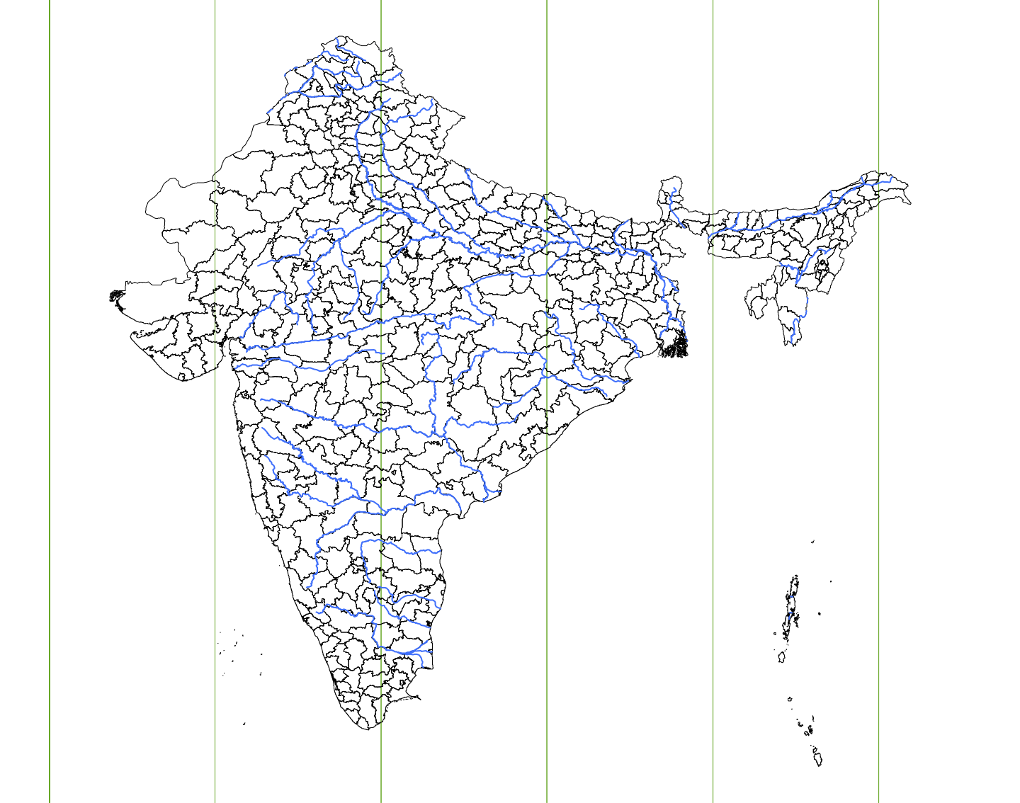
For large areas such as India:
No single map projection preserves distance in every direction
$\Rightarrow$ Project each district to appropriate UTM projection
$\Rightarrow$ Loop over UTM zone numbers
India with UTM Zones
Exercise #4
Calculate river length by district
1. Assign UTM zone number to each river-by-district
2. Extract rivers whose centroid is within each UTM zone
3. Project to UTM
4. Calculate river length by district
5. Loop over steps 2-4 for all UTM zone numbers
$\Rightarrow$ Use Model Builder first, then edit the exported Python script to create a loop.
Exercise #4.1: Overview
Assign UTM zone number
Inputs:
river_by_district.shp (created in Exercise #2)
utm.shp: UTM zone polygons, provided by ArcGIS
- The file is located in C:\Program Files (x86)\ArcGIS\Desktop10.6\Reference Systems
- The version number may differ from 10.6
- Right-click Folder Connections to access to this directory
Exercise #4.1: Overview (cont.)
Geo-processing tools:
1. Feature To Point (cf. Lecture 4)
- Some rivers may cross UTM zone boundaries
- Assign UTM zone number based on centroid
2. Spatial Join
- Match river centroids with UTM zone polygons
3. Copy Features + Join Field
- Transfer UTM zone number in centroid table to river table
- Join Field overwrites the input
- So copy river features first
Exercise #4.1: Overview (cont.)
There is a tool called "Calculate UTM Zone"
But it's not useful at all.
- It creates a new field that contains the full string of the coordinate system, which may be truncated...
- Why doesn't it just give the UTM zone number???
Now open the empty model exercise4
It's best to separate a model from the one for Exercises 1-3
- Each model (and Python script) should deal with one single purpose
- Otherwise your coauthors and your future self will get confused
Exercise #4.1
Feature To Point
Input Features: ...\output\river_by_district.shp
Output Feature Class: ...\temporary\river_centroids.shp
Uncheck "Inside"
- We need the average location for each river, not the point on river
Exercise #4.1 (cont.)
Spatial Join
Target Features: river_centroids.shp
- Output from Feature To Point
Join Features: C:\Program Files (x86)\ArcGIS\Desktop10.6\Reference Systems\utm.shp
Output Feature Class: ...\Lecture6\temporary\utm_zones.shp
Spatial Join (cont.)
Join Operation: JOIN_ONE_TO_ONE
Check "Keep All Target Features"
Field Map of Join Features: leave as it is
- We handle this in Python later
Match Option: Intersect
Exercise #4.1 (cont.)
Copy Features
- To prepare for using Join Field
Input Features: river_by_district.shp
Output Feature Class: ...\Lecture6\temporary\river_utm.shp
Join Field
Add fields from another shapefile's attribute table
-
Very much the same as Stata's
merge
Overwrites the input. So use Copy Features first.
Exercise #4.1 (cont.)
Join Field
Input Table: river_utm.shp
- Output from Copy Features
Input Join Field: GID_2
Join Field (cont.)
Join Table: utmzones.shp
- Output from Spatial Join
Output Join Field: GID_2
- Name of field in Join Table, to be used for joining
Join Field(s): check ZONE
- Field for UTM zone number
NOTE: This tool overwrites the input data.
Join Field to add your own data
Create your data as a csv file
Then use Table to Table, to convert it into dBASE format.
Finally, use Join Field
We will learn this in Lecture 7
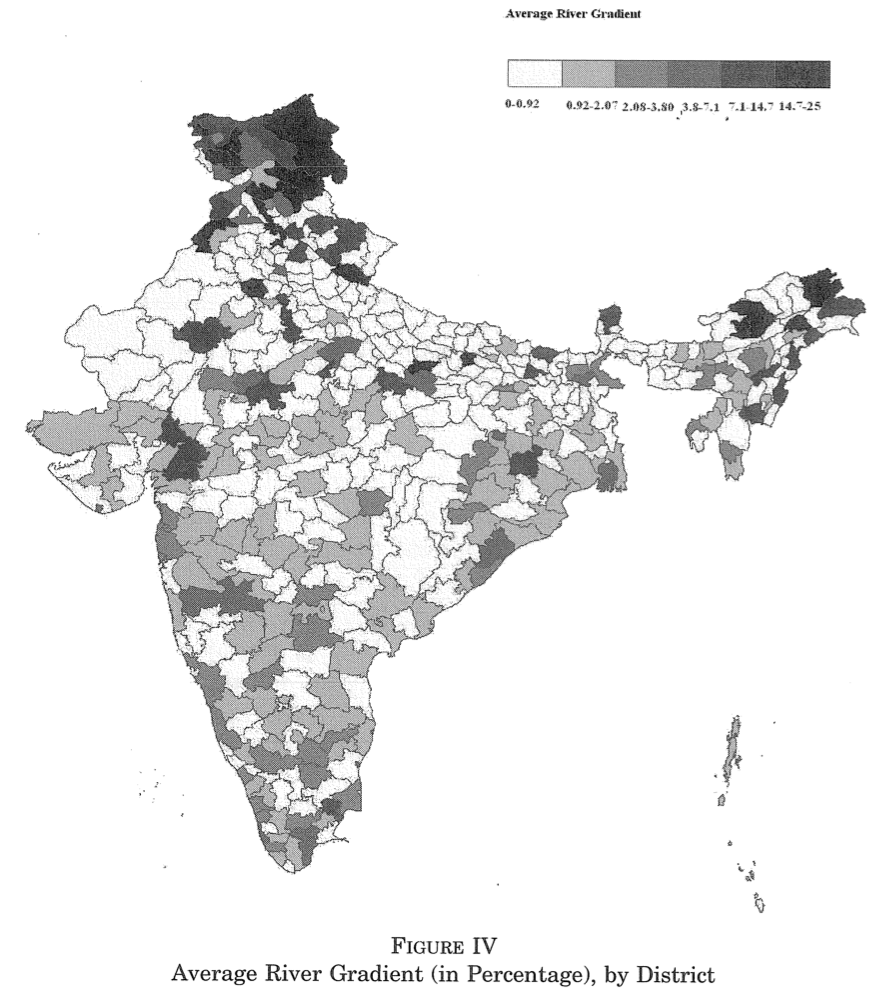
Assignment #2
Mean river gradient map of India
Replicate Figure IV of Duflo & Pande (2007)
Exercise #4.2: Overview
Extract rivers by UTM zone
Geo-processing tool: Select (Analysis)
This tool keeps features whose field values satisfy the conditions you specify
Useful in various situations
- Keep unmatched areas from Union (cf Lec 5)
- Sample selection (e.g. select India from global data)
Exercise #4.2
Select (Analysis)
Input Features: river_utm.shp (2)
- Output from Join Field
Output Feature Class: ...\Lecture6\temporary\river43.shp
Expression: "ZONE" = 43
- Field name: must be enclosed by ""
- See ArcGIS Help on SQL reference to learn other syntax rules
Exercise #4.3
Project to UTM
Which geo-processing tool(s) should we use?
Exercise #4.3 (cont.)
Project
Input Dataset or Feature Class: river43.shp
- Output from Select
Output Dataset or Feature Class: ...\temporary\river43_projected.shp
Output Coordinate System: WGS_1984_UTM_Zone_43N
Exercise #4.4
Calculate river length
Geo-processing tools: Add Geometry Attributes
cf. Surface area calculation (Lecture 4)
Exercise #4.4 (cont.)
Add Geometry Attributes
Input Features: river43_projected.shp
- Output from Project
Geometry Property: LENGTH
Length Unit: METERS
NOTE: This tool overwrites the input data.
Exercise #4.5
Table To Excel
Input Table: river43_projected.shp (2)
- Output from Add Geometry Attributes
Output Excel File: ...\Lecture6\output\river_length43.xls
An alternative to Exercise #4.3 and #4.4
You can directly use Add Geometry Attributes (cf. Lecture 4)
Input Features: river43.shp
- Output from Select
Geometry Properties: LENGTH_GEODESIC
Area Unit: METERS
Coordinate System: WGS_1984_UTM_Zone_43N
- If unspecified, the area is calculated based on WGS 1984 (i.e. rubbish)
Get ready for Python coding
Now export the model exercise4 as a Python script
Open both the exported script and the template script (code/template4L6.py) with IDLE
We first review what we have learned (cf Lecture 2)
Then we create a loop over UTM zones
Use Try-Except statement (review)
- For printing error messages
1. Copy geo-processing commands in exported script
2. Paste them below try: in template script
3. Select them all
4. Indent them by pressing the tab key
Assign variables to file names (review)
- For ease of understanding/editing the script later
1. Copy local variables in exported script
2. Paste them above try: in template script
3. Sort them by inputs, intermediate files, and outputs
-
Inputs:
temporary\\river_by_district.shp,...\\utm.shp -
Outputs:
output\\river_length43.xls
Assign variables to file names (cont.)
4. Specify the working directory (see Lecture 3)
arcpy.env.workspace = "../"
5. Remove directory path from file names
utm_zones_shp = "C:\\...\\utm_zones.shp"
$\Downarrow$
utm_zones_shp = "temporary\\utm_zones.shp"
Assign variables to file names (cont.)
6. Replace duplicated variables
- Model Builder duplicates variables for outputs from overwriting tools (Join Field, Add Geometry Attributes)
- Press ctrl + f (for IDLE, Edit > Replace), to avoid mistakes
rivers_utm_shp___2_
$\rightarrow$ rivers_utm_shp
river43_projected_shp___2_
$\rightarrow$ river43_projected_shp
Spatial Join in Python
Replace the lengthy 6th argument with ""
- Otherwise, field GID_2 may become all 0 for some reason...
Whenever using Spatial Join in Python, make sure the 6th argument is empty.
5. Loop over values in Python
Exercise #4.6: Overview
Loop over UTM zones
Put the following geo-processing steps into a loop
- Select, Project, Add Geometry Attributes, Table To Excel
At each turn of loop, change:
1. UTM zone number for Select
"\"ZONE\" = 43"
2. UTM coordinate system for Project
3. Output file names
Exercise #4.6: Overview (cont.)
Create a loop over values from 43 to 47
- India ranges from UTM zone 42 to 47
- There is no river in zone 42
To do so, add the following command line
for zone in range(43,48):
Loop over numbers in Python
for zone in range(43,48):
This command line does the following:
1. Creates a variable zone that contains number 43
2. Executes all the indented commands below
3. Then assigns next number (44) to zone
4. Executes all the indented commands below
5. Repeats this until number 47 (not 48!)
Loop over numbers in Python (cont.)
Same can be done by the while loop
zone = 43
while zone < 48:
    commands
    zone = zone + 1
or the list loop (to be used in Lecture 7)
zoneList = [43,44,45,46,47]
for zone in zoneList:
    commands
Exercise #4.6 (1)
Create a loop structure in script
1. Add:
for zone in range(43,48):
arcpy.Select_analysis...
2. Indent the four geo-processing commands
Now the code should look like this:
for zone in range(43,48):
  # Process: Select
  arcpy.Select_analysis(...)
  # Process: Project
  arcpy.Project_management(...)
  # Process: Add Geometry Attributes
  arcpy.AddGeometryAttributes_management(...)
  # Process: Table To Excel
  arcpy.TableToExcel_conversion(...)
Exercise #4.6 (2)
Select a UTM zone number
Let's first understand the syntax for Select tool
Syntax for Select tool
arcpy.Select_analysis(river_utm_shp, river43_shp, "\"ZONE\"=43")
1st argument: input file name
Syntax for Select tool
arcpy.Select_analysis(river_utm_shp, river43_shp, "\"ZONE\"=43")
2nd argument: output file name
Syntax for Select tool
arcpy.Select_analysis(river_utm_shp, river43_shp, "\"ZONE\"=43")
3rd argument: selection rule
Syntax for selection rule
"\"ZONE\"=43"
Must be string, thus enclosed by " "
Syntax for selection rule
"\"ZONE\"=43"
Field name must be enclosed by \" \"
- " " is used by Python as string enclosure
- For Python to read " as field name enclosure, add backslash \
Syntax for selection rule
"\"ZONE\"=43"
We want to replace this number at each turn of the loop
To do so, write as follows:
"\"ZONE\"="+str(zone)
Number vs String
"\"ZONE\"="+str(zone)
Variable zone contains number, not string
But selection rule expression has to be string
Convert Number into String
"\"ZONE\"="+str(zone)
So transform number into string by str( )
Concatenate strings
"\"ZONE\"="+str(zone)
To "concatenate" (i.e. connect) two strings, use +
Concactenate strings
"\"ZONE\"="+str(zone)
Don't forget to enclose a string with " "
Summary (1/4)
"\"ZONE\"="+str(zone)
We have two strings
Summary (2/4)
"\"ZONE\"="+str(zone)
We have two strings concatenated by +
Summary (3/4)
"\"ZONE\"="+str(zone)
Number must be converted into string by str()
Summary (4/4)
"\"ZONE\"="+str(zone)
Field name must be enclosed by \" \"
Exercise #4.6 (2)
Replace the 3rd argument for the Select tool
"\"ZONE\"= 43"
with
"\"ZONE\"="+str(zone)
Exercise #4.6 (3)
Specify UTM projection
Let's first understand the syntax for Project tool
Syntax for Project tool
arcpy.Project_management(river43_shp, river43_projected_shp, "PROJCS[...
1st argument: input file name
Syntax for Project tool
arcpy.Project_management(river43_shp, river43_projected_shp, "PROJCS[...
2nd argument: output file name
Syntax for Project tool
arcpy.Project_management(river43_shp, river43_projected_shp, "PROJCS[...
3rd argument: coordinate system name
(too long to be shown in this slide)
Specify coordinate system in Python
Use factory code (unique ID for each coordinate system)
UTM projections for zones 43-47:
32643, 32644, 32645, 32646, 32647
Then use SpatialReference method
SpatialReference method
factorycode = 32643
cs = arcpy.SpatialReference(factorycode)
arcpy.Project_management(river43_shp, river43_projected_shp, cs)
Create a variable for factory code
SpatialReference method
factorycode = 32643
cs = arcpy.SpatialReference(factorycode)
arcpy.Project_management(river43_shp, river43_projected_shp, cs)
SpatialReference method takes factory code as input
SpatialReference method
factorycode = 32643
cs = arcpy.SpatialReference(factorycode)
arcpy.Project_management(river43_shp, river43_projected_shp, cs)
Then returns that long string name for coordinate system
SpatialReference method
factorycode = 32643
cs = arcpy.SpatialReference(factorycode)
arcpy.Project_management(river43_shp, river43_projected_shp, cs)
We assign variable cs to coordinate system name
SpatialReference method
factorycode = 32643
cs = arcpy.SpatialReference(factorycode)
arcpy.Project_management(river43_shp, river43_projected_shp, cs)
Use it as 3rd argument for Project
SpatialReference method in loop
for zone in range(43,48):
factorycode = 32600 + zone
cs = arcpy.SpatialReference(factorycode)
arcpy.Project_management(river43_shp, river43_projected_shp, cs)
Then use variable zone to change factory code for each turn of the loop
- Factory code must be number, not string
-
So don't use
str(zone)
Exercise #4.6 (3)
Modify the script as follows (marked in yellow)
for zone in range(43,48):
arcpy.Select_analysis(river_utm_shp, river43_shp, "\"ZONE\" = " + str(zone))
factorycode = 32600 + zone
cs = arcpy.SpatialReference(factorycode)
arcpy.Project_management(river43_shp, river43_projected_shp, cs)
Exercise #4 Step 5 (4)
Output file names
Select the names of files to be created within loop
Cut-and-paste them to beginning of loop
for zone in range(43,48):
river43_shp = "river43.shp"
river43_projected_shp = "river43_projected.shp"
river_length43_xls = "river_length43.xls"
Don't forget indenting them
Output file names
Replace 43 in the file names with "+str(zone)+"
- Do not change variable names!
for zone in range(43,48):
river43_shp = "rivers"+str(zone)+".shp"
river43_projected_shp = "rivers_pj"+str(zone)+".shp"
river_length43_xls = "river_length"+str(zone)+".xls"
This way, each turn of the loop will create different files
Exercise #4 Step 5 (5)
Print commands
To explain what each command line does, add:
print "..."
- This allows you to monitor which part of the script is being run
-
What follows after
printmust be a string - You can use string variables
Print commands (cont.)
To indicate each turn of the loop:
for zone in range(43,48):
    print "Processing UTM zone "+str(zone)
Another example of string concatenation
Now run the script by pressing F5 in IDLE
Model Python Script for Exercise 4
Look at solutions4exercises/exercise4.py
What we've learned on ArcGIS
- Covert elevation raster into gradient raster
- Create indicator raster
- Attach UTM zone numbers to features
- Calculate length of polyline features
Do you remember which geo-processing tools you used for each of these tasks?