Causal Inference with Spatial Data
(ArcGIS 10 for Economics Research)
Lecture 5
Zonal Statistics
Masayuki Kudamatsu
9 November, 2018
Press SPACE to proceed.
To go back to the previous slide, press SHIFT+SPACE.
What is Zonal Statistics?
Summary statistics of raster data value within each polygon
i.e. Merge polygons with raster data
Examples:
- Indonesian districts + Forest coverage (Lecture 1)
- Grid cells + Population counts
- Population weights for averaging grid-cell temperature to country (Dell et al. 2012)
What is Zonal Statistics? (cont.)
More examples:
Mean nighttime luminosity within:
- Country (Henderson et al. 2012)
- Provinces (Hodler & Raschky 2014)
- Electoral districts (Baskaran et al. 2015)
- Ethnic homelands (Michalopoulos & Papaioannou 2013 / 2014, Alesina et al. 2016)
What is Zonal Statistics? (cont.)
The following summary statistics can be obtained:
- Mean / Standard deviation
- Min / Max / Range
- Sum
- Count
For integer rasters only:
- Median
- Variety (# of unique values)
- Majority (most frequent value)
- Minority (least frequent value)
An application of Zonal Statistics for research design
Michalopoulos (2012): probably the most ingenious application of zonal statsitics (and ArcGIS in general)
Today's road map
1. Michalopoulos (2012)
2. Virtual country data
- Intersect + Dissolve
- Zonal Statistics as Table
3. Adjacent cell pair data
- Extract Multi Values To Points
- Polygon Neighbors
1. Michalopoulos (2012)
Research Question
Did geographic diversity cause ethnic diversity?
Important?
- Ethnic diversity: known to "cause" low growth (Easterly & Levine 1997) and conflict (Montalvo & Reynal-Querol 2005)
Original?
- Cross-"virtual country" regression
Feasible?
Data
Spatial distribution of languages
- Source: World Lanugage Mapping System
- Polygons of linguistic groups' homelands, 1990-95
Suitability for agriculture (Ramankutty et al. 2002)
- Raster at 0.5° x 0.5° resolution
- Fraction of a cell cultivable around 1990
- Obtained by "regressing" observed cultivated areas (satellite images) on climate and soil
Elevation and other geography variables
Empirical challenge
Omitted variable bias in cross-country regression
- Countries with centralized modern state may have both homogenized languages & conquered homogenous areas
Panel data analysis: infeasible
- Geography: time-invariant
Empirical challenge (cont.)
Global raster data allows for sub-national district analysis
- Can control for country FE
But... sub-national district boundaries: endogenous
- Maybe difficult to split districts by ethnicity if geography is diverse
Empirical challenge (cont.)
Solution 1: cross-"virtual country" regression
- Divide the earth into 2.5° x 2.5° grid cells
- Boundary thus exogeneous
Solution 2: Dyadic regression
- Pair each raster cell with one of its 8 adjacent cells
- Measure differences within each pair
- Can control for raster cell FE
Neither is feasible w/o GIS
Virtual country example
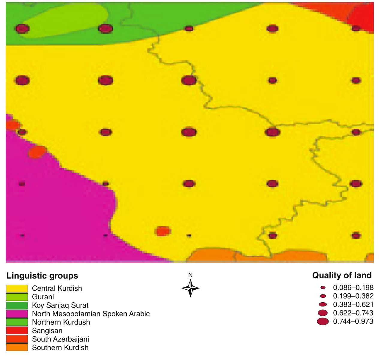
Figure 7 of Michalopoulos (2012)
Cross-"virtual country" regression
\begin{align*} ln(\#Languages_i) = & \ \beta_0 + \beta_1 Latitude_i \\ & + \beta_2 SD(Elevation)_i \\ & + \beta_3 SD(LandQuality)_i \\ & + \boldsymbol{x}'_{i}\boldsymbol{\beta_4} + \varepsilon_{i} \end{align*}
| $Latitude_i$ | Literature has found its association w/ ethnic diversity |
| $\boldsymbol{x}_i$ | Vector of controls (country FE, etc.) |
We will learn how to calculate $SD(LandQuality)_i$
Standard errors
Clustered at country level
Conley's (1999) method can also be used (cf. Lec 3)
- With Hsiang's (2010) Stata code, geographic coordinates can now be used
Results (table 4 columns 4-6)
| Dependent Variable: ln(# of languages) | ||||
| Sample | All | Tropics | Non-tropics | |
|---|---|---|---|---|
| SD(land quality) | 0.116*** | 0.103** | 0.173*** | |
| [0.033] | [0.048] | [0.055] | ||
| SD(elevation) | 0.082*** | 0.118** | 0.093** | |
| [0.030] | [0.057] | [0.043] | ||
| Country FE | YES | YES | YES | |
| Other controls | YES | YES | YES | |
| # observations | 1663 | 536 | 1127 | |
| Standard errors clustered at country level. | ||||
| * significant at 10%, ** 5%, *** 1%. | ||||
Dyadic regression
Unit of analysis: pair of neighboring cells $ij$
\begin{align*} \%CommonLanguages_{ij} = & \ \gamma_0 + \gamma_1 \Delta(LandQuality)_{ij} \\ & + \gamma_2 \Delta(Elevation)_{ij} \\ & + \boldsymbol{x}'_{ij}\boldsymbol{\gamma_3} + \mu_i + \nu_j + \xi_{ij} \end{align*}
| $\mu_i, \nu_j$ | Cell FEs for $i$ and $j$ |
Results (table 6 columns 2-5)
| Dependent Variable: % Common Languages | ||||
| Sample | All | Africa | Europe | Asia |
|---|---|---|---|---|
| $\Delta$LandQuality | -0.038*** | -0.054*** | -0.048** | -0.056*** |
| [0.012] | [0.018] | [0.021] | [0.016] | |
| $\Delta$Elevation | -0.051*** | -0.050*** | -0.046** | -0.053*** |
| [0.006] | [0.016] | [0.022] | [0.009] | |
| Cell FE | YES | YES | YES | YES |
| Controls | YES | YES | YES | YES |
| Observations | 156570 | 35305 | 11975 | 74830 |
| Standard errors clustered at country level. | ||||
| * significant at 10%, ** 5%, *** 1%. | ||||
Prepare for the rest of this lecture
1. Launch ArcMap 10 (it takes time)
2. Download the zipped dataset for Lecture 5
3. Save it to Desktop (C:\\Users\\yourname\\Desktop)
- Don't save in the remote server, which slows down ArcGIS
4. Right-click it and choose 7-Zip > Extract to "Lecture5\"
-
So the directory path will be:
C:\\Users\\yourname\\Desktop\\Lecture5
Prepare for the rest of this lecture (cont.)
In the input/ folder...
5a. Right-click suit.zip (agricultural suitability raster) and choose 7-Zip > Extract to "suit\"
- This is a raster data in ESRI grid format.
- The directory structure for grid raster is very complicated
- Keep every file in one subfolder to avoid confusion when browsed in File Explorer
5b. Right-click the following zipped data and choose 7-Zip > Extract Here
-
gadm36_0.zip(country polygons) -
GREG.zip(ethnolinguistic group polygons)
Prepare for the rest of this lecture (cont.)
Now in ArcMap's Catalogue Window:
6. Establish connection to data folder
- Right-click Folder Connections
- Select Connect to Folder
- Choose Desktop > Lecture5
7. Prepare the Model Builder
Data Cleaning 1: GREG
Browse GREG.shp (Geo-referencing of Ethnic Groups data)
- We use this data because World Language Mapping System data is not for free
Same language group split into several polygons if:
- Inhabiting non-adjacent areas
- Cohabitated with other language groups
$\Rightarrow$ Three fields for language group code/name
In this lecture, we assume each polygon represents one language group
Data Cleaning 1: GREG (cont.)
For how to make each language has only one polygon, see:
Model: solutions4exercises/models.tbx/cleanGREG
Python script: solutions4exercises/cleanGREG.py
Data Cleaining 2: Suitability for Agriculture
Now browse the "suitability for agriculture" raster data
It has no coordinate system assigned.
We need to assign it ourselves, by looking at the meta data
- But... There is no meta data to tell what coordinate system should be assigned
- So we assume it's WGS 1984
- (We should avoid using such spatial data...)
Which geo-processing tool(s) should we use?
Data Cleaining 2: Suitability for Agriculture (cont.)
Since Define Projection overwrites the input file, we should make a copy
The Copy Features tool works only with vector data
For raster data, we use the Copy Raster tool
So let's edit models.tbx/cleandata
Data Cleaining 2: Suitability for Agriculture (cont.)
Copy Raster
Input Raster: ...\Lecture5\input\suit\suit
Output Raster Dataset: ...\Lecture5\output\landquality.tif
- By adding ".tif", we will save the raster in the TIFF format
Data Cleaining 2: Suitability for Agriculture (cont.)
Without running the model, export and edit a Python script. Then run the script.
Model Python script: solutions4exercise/cleandata.py
2. Virtual Country Data
Data we want to construct
Unit of observations: Virtual country polygons
- 2.5° x 2.5° cell's region with language data available (see p. 1516)
Dependent variable: # of languages spoken
Regressor: Standard deviation of land quality
We now create these data by editing exercises1-3
Exercise #1: Overview
Virtual country polygons
Geo-processing tools:
1. Create Fishnet + Define Projection (cf. Lecture 2)
- Creates 2.5° x 2.5° cells
2. Add Field + Calculate Field
- Assign the unique ID in the attribute table
Exercise #1: Step 1
Create Fishnet
Output Feature Class: ...\Lecture5\temporary\fishnet25.shp
Template Extent (see p. 1522)
Top: 85
Left: -180
Right: 180
Bottom: -65
$\Rightarrow$ Automatically fill in Fishnet Origin Coordinate and Y-Axis Coordinate
Create Fishnet (cont.)
Cell Size Width: 2.5
Cell Size Height: 2.5
Number of Rows: 0
Number of Columns: 0
$\Rightarrow$ Automatically calculate # of rows/columns given the extent and cell size
Create Fishnet (cont.)
Uncheck "Create Label Points"
- Label points: unnecessary for our purpose
- Model Builder will still show label points as an output from Create Fishnet. This is a bug.
Geometry Type: POLYGON
- By default, this option is set as POLYLINE. Make sure to change it.
Exercise #1: Step 1 (cont.)
What coordinate system should we assign to the fishnet?
Same one as other spatial datasets
$\Rightarrow$ Check the coordinate system of GREG
- How? Review Lecture 1
Exercise #1: Step 1 (cont.)
Define Projection (Data Management)
Input Dataset or Feature Class: fishnet25.shp
Coordinate System: GCS_WGS_1984
- Geographic Coordinate Systems > World > WGS 1984
- This is the coordinate system used by GREG
NOTE: This tool overwrites the input data.
Exercise #1 Step 1 (cont.)
Now save and run the Model.
Browse the attribute table of fishnet25.shp.
Fields created:
-
FID: unique integer identifier starting from 0 -
Id: all values are 0...
Exercise #1 Step 2
We need virtual country ID for merging data in Stata
Field name FID is used for every shapefile...
$\Rightarrow$ Create your own ID for virtual countries
To create a new field, we need two tools:
- Add Field
- Calculate Field
Exercise #1: Step 2 (cont.)
Add Field
Input Table: fishnet25.shp (2)
- Output from Define Projection
Field Name: cell25_id
- Or whatever you prefer (not exceeding 10 characters)
Field Type: SHORT
- We create integer identifier
- Total # of cells: 8640
NOTE: This tool overwrites the input data.
Exercise #1: Step 2 (cont.)
Calculate Field
Input Table: fishnet25.shp (3)
- Output from Add Field
Field Name: cell25_id
- Or the same as what you specified in Add Field
Calculate Field (cont.)
Expression: !FID! + 1
- ! ! tells Python what's enclosed is a field name
- You don't have to add 1
- But ID usually starts from 1
Expression Type: PYTHON_9.3
NOTE: This tool overwrites the input data.
Exercise #1 Step 2 (cont.)
Now save and run the Model.
Browse the output attribute table.
Is everything as expected?
Exercise #2: Overview
# of languages spoken
Simplest approach: Spatial Join (JOIN_ONE_TO_MANY)
- Match each virtual country w/ all intersecting language polygons
- Then export the table to Stata
-
collapse (count) ..., by(cell25_id)
Exercise #2: Overview (cont.)
# of languages spoken
Alternative approach: Intersect + Dissolve
- Intersect throws away the area of a virtual country that's not overlapped w/ language polygons
- Dissolve merges all language polygons w/i each virtual country
Michalopoulos (2012, p. 1516): "... geographic measures are calculated focusing on regions with linguistic coverage ..."
$\Rightarrow$ Preferred approach in this context
Also allows you to create a map of # of languages spoken
Exercise #2: Step 1
Intersect (Analysis)
Input Features:
-
...\Lecture5\input\GREG.shp - fishnet25.shp (4)
Output Feature Class: ...\Lecture5\temporary\intersect.shp
Join Attributes: ALL
Output Type: INPUT
Exercise #2: Step 2
Dissolve (Analysis)
Input Features: intersect.shp
Output Feature Class: ...\Lecture5\temporary\vcountry.shp
Dissolve_Field(s): cell25_id
Statistics Field(s): FID_GREG
Statistic Type: COUNT
Check "Create multipart features"
- Otherwise non-contiguous polygons won't be dissolved
Exercise #2 (cont.)
Now save and run the Model.
To check if # of languages spoken is properly calculated:
-
Browse
fishnet25.shp(make polygon color unfilled) - Select (say) cell_id 1340 in attribute table
- Right-click fishnet25.shp and choose "Selection > Zoom To Selected Features"
- Now count # of polygons in GREG.shp within this cell
-
Browse attribute table of
vcountry.shp - For cell_id 1340, COUNT_FID has a value of 4?
$\Rightarrow$ It's 4
Exercise #2 (cont.)
Polygons in GREG.shp are slightly overlapping over each other
-
Zoom in a lot to the boundaries of
GREG.shp
$\Rightarrow$ Intersect creates tiny polygons along the border
Solution: set XY Tolerance a little bit higher in the Intersect tool
XY Tolerance
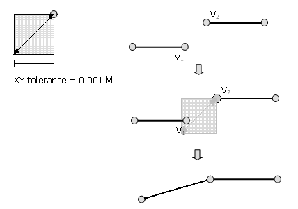
Size of a square treated as a point in geo-processing
Default: 0.001 meters
XY Tolerance (cont.)
Increasing XY Tolerance a bit (say, to 1 meter) usually solves the problem of Intersect, Spatial Join etc.
CORRECTION
Exercise #2: Step 1
Intersect (Analysis)
Input Features: GREG.shp, fishnet25.shp (3)
Output Feature Class: ...\Lecture5\temporary\intersect.shp
Join Attributes: ALL
XY Tolerance: 1 Meters
Output Type: INPUT
Application of Intersect + Dissolve
Hoxby (2000)
Does competition improve school quality?
# of streams within city: IV for # of school districts
- Intersect streams w/ metropolitan areas
- Dissolve by metropolitan area
Similar idea was used by Bai and Jia (2016)
Exercise #3: Overview
Standard deviation of land quality
Inputs:
- Virtual country polygons (with language data available)
- Suitability for Agriculture raster
Geo-processing tool: Zonal Statistics as Table
Zonal Statistics as Table
Creates a table where
- Each row: polygon zone
- Columns: zonal statistics
Output is NOT the attribute table to input polygons
- Use Table To Excel, to export
Don't confuse with another tool called Zonal Statistics
- Creates a raster data, instead of a table
Cannot use Zonal Statistics as Table? See next slide:
Spatial Analyst extension
Zonal Statistics as Table is part of the Spatial Analyst extension.
- This extension allows us to work on raster datasets
By default, you're not allowed to use it.
To activate, click in the menu bar Customize > Extensions... and check Spatial Analyst
- Same for other extensions
Exercise #3: Step 1
Zonal Statistics as Table
Input raster or feature zone data: vcountry.shp
- Output from Dissolve
Zone field: cell25_id
Input value raster: output/landquality.tif
- Output from data cleaning we did
- Use the directory icon, not drop-down menu
Zonal Statistics as Table (cont.)
Output table: ...\Lecture5\temporary\landquality25.dbf
- Adding ".dbf" will create a table in the dBASE format
Check "Ignore NoData in calculations"
- If unchecked, zonal statistics is missing if there is at least one raster cell with NoData
Statistics type: ALL
- STD: main regressor
- MEAN: control
- RANGE: robustness check (Table 5B column 3)
Exercise #3 Step 2
Table To Excel
- Input Table: landquality25.dbf
-
Output Excel File:
...\Lecture5\output\landquality25.xls
Here we cannot use Export Feature Attribute to ASCII
- Zonal Statistics as Table creates a table, not a feature class
- Export Feature Attribute to ASCII only takes a feature class as the input
Exercise #3 (cont.)
Now save and run the Model.
Browse the output Excel file.
OID: just the row ID
cell25_id: use this to merge in Stata
COUNT: # of raster cells used for calculation
- Used for sample selection (at least 10; see p. 1524)
AREA: in degrees and thus useless
Extra
Data for Table 3
How to obtain zonal stats for areas without language data?
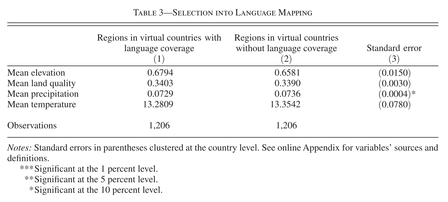
Data for Table 3 (cont.)
Solution:
Union + Select + Zonal Statistics as Table
- Union: same as Intersect except for keeping unmatched features (as multipart features)
- If unmatched, FID_GREG = -1
- Select: keep features by their attritubes (cf. Lecture 6)
- Keep those with FID_GREG = -1
"Model" model for Exercises 1-3
See models.tbx\exercises1-3
in the solutions4exercises\ folder
Assignment #1
Sample selection by population
"In the regression analysis, virtual countries of at least 3,000 inhabitants are included." (p. 1523)
$\Rightarrow$ Obtain population for each virtual country
- Use population raster by Gridded Population of the World
- Then which geo-processing tool should you use?
Assignment #2
# of countries in each virtual country
Which geo-processing tool(s) should you use?
Assignment #3
Other control variables
Reviewing Lecture 4 allows you to create:
1. Absolute latitude
2. Migratory distance from East Africa (hint)
- See p.10 of Data Appendix for detail
3. Surface area (hint)
4. Sea distance (hint)
5. Water area (hint)
3. Adjacent cell pair data
Data we want to construct
1. Data at 0.5°x0.5° cell level
2. List of adjacent cell pairs
- Unit of observations
Exercise #4: Overview
0.5° x 0.5° cell data
1. Create cell polygons (cf. Exercise 1)
2. Extract language spoken
3. Extract land quality
Exercise #4: Step 1 (1)
Create Fishnet
Output Feature Class: ...\Lecture5\temporary\fishnet05.shp
Template Extent
Top: 85
Left: -180
Right: 180
Bottom: -65
$\Rightarrow$ Automatically fill in Fishnet Origin Coordinate and Y-Axis Coordinate
Create Fishnet (cont.)
Cell Size Width: 0.5
Cell Size Height: 0.5
Number of Rows: 0
Number of Columns: 0
$\Rightarrow$ Automatically calculate # of rows/columns given the extent and cell size
Create Fishnet (cont.)
Uncheck "Create Label Points"
- Label points: unnecessary for our purpose
- Model Builder will still show label points as an output from Create Fishnet. This is a bug.
Geometry Type: POLYGON
- By default, this option is set as POLYLINE. Make sure to change it.
Exercise #4: Step 1 (2)
Define Projection (Data Management)
Input Dataset or Feature Class: fishnet05.shp
Coordinate System: GCS_WGS_1984
- Geographic Coordinate Systems > World > WGS 1984
- This is the coordinate system used by GREG
NOTE: This tool overwrites the input data.
Exercise #4: Step 1 (3)
Add Field
Input Table: fishnet05.shp (2)
- Output from Define Projection
Field Name: cell05_id
- Or whatever you prefer (not exceeding 10 characters)
Field Type: LONG
- Total # of cells: 216,000
- SHORT cannot handle values larger than 32,767
Exercise #4: Step 1 (4)
Calculate Field
Input Table: fishnet05.shp (3)
- Output from Add Field
Field Name: cell05_id
- Or the same as what you specified in Add Field
Calculate Field (cont.)
Expression: !FID! + 1
- ! ! tells Python what's enclosed is a field name
Expression Type: PYTHON_9.3
NOTE: This tool overwrites the input data.
Exercise #4 Step2
Extract language spoken
Use Spatial Join
- Name (or code) of languages needed to obtain % of common languages within a pair of adjacent cells
When exported to Stata, execute:
bysort cell05_id: gen id = _n
reshape wide ..., i(cell05_id) j(id)
to make one row per cell
Exercise #4 Step2 (cont.)
Spatial Join
Target Features: fishnet05.shp (4)
- Output from Calculate Field
Join Features: ...\Lecture5\input\GREG.shp
Output Feature Class: ...\Lecture5\temporary\cell05.shp
Join Operation: JOIN_ONE_TO_MANY
Uncheck "Keep All Target Features"
- Drops all the cells without language data
Exercise #4 Step3
Extract land quality
We could use Zonal Statistics as Table
But each polygon has only one raster cell
Here we take alternative approach:
- Feature To Point
- Extract Multi Values To Points
Extract Multi Values To Points
Extract raster values from the cell below the point feature
Value -9999 will be assigned if no raster data
This tool also overwrites the input attribute table
cf. Another tool Extract Values To Points does the same thing, but one raster at a time (and field name cannot be chosen)
Exercise #4: Step 3 (1)
Feature To Point
Input Features: cell05.shp
- Output from Spatial Join
- We don't need cells where no language is spoken
Output Feature Class: ...\Lecture5\temporary\cell05centroids.shp
Uncheck "Inside"
Exercise #4: Step 3 (2)
Extract Multi Values To Points
Input point features: cell05centroids.shp
- Output from Feature To Point
Input rasters: landquality.tif
Output field name: land_q
- Field name cannot be longer than 10 characters
Exercise #4: Step 4
Export data to Stata
We cannot use Table to Excel
- # of cells: more than Excel's limit of 65535
$\Rightarrow$ use Export Feature Attributes to ASCII
Exercise #4: Step 4 (cont.)
Export Feature Attribute to ASCII
Input Feature Class: cell05centroids.shp (2)
Value Field: cell05id, G1ID, G2ID, G3ID, land_q
Delimiter: SPACE
- Not COMMA, to avoid confusing with decimal mark
Output ASCII File: ...\Lecture5\output\cell05.txt
Check "Add Field Name to Output"
Exercise #5
List of adjacent cell pairs
Inputs: 0.5° x 0.5° cell polygons (cf. Exercise #4)
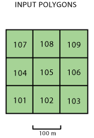
Geo-processing tools: Polygon Neighbors
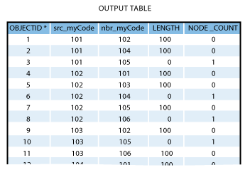
Polygon Neighbors
Application of Polygon Neighbors
Acemoglu et al. (2015)
State capacity in one municipality
$\Rightarrow$ State capacity & prosperity in neighboring municipalities
- Polygon Neighbors: identify neighboring municipalities among 1017 in total in Colombia
Exercise #5 Step 1
Polygon Neighbors
Input Features: cells05.shp
- Output from Spatial Join
Output Table: ...\Lecture5\temporary\cell_neighbors.dbf
Report By Field(s): check cell05_id
Uncheck "Include both sides of neighbor relationship"
- Otherwise each pair is observed twice
- Check if unit of analysis is the cell, not the pair (e.g., Acemoglu et al. 2015)
Exercise #5 Step 2
Export table with many rows
Run the tool and browse the table
Notice # of rows more than Excel's limit of 65535
$\Rightarrow$ Table to Excel does not work
ArcGIS has no tool to export table as a text file
What should we do?
Export table with many rows (cont.)
Solution: Table Select
This tool picks a subset of rows from the input table
$\Rightarrow$ Divide the table into several
Exercise #5 Step 2 (1)
Table Select
Input Table: cell_neighbors.dbf
Output Table: ...\Lecture5\temporary\cell_neighbors1.dbf
Expression: "OID" < 65000
- "OID": row #
Exercise #5 Step 2 (2)
Table Select
Input Table: cell_neighbors.dbf
Output Table: ...\Lecture5\output\cell_neighbors2.dbf
Expression: "OID" >= 65000 AND "OID" < 130000
And so on until all rows are covered.
Then finally...
Exercise #5 Step 3
Table to Excel
Input Table: cell_neighbors1.dbf
Output Excel File: ...\Lecture5\output\cell_neighbors1.xls
And so on, and append them in Stata
"Model" model for Exercises 4-5
Look at models.tbx\exercises4-5
in the solutions4exercises\ folder
Python: Check Out Extension
When using Spatial Analyst extension tools...
- Zonal Statistics as Table
- Extract Multi Values To Points
Make sure you add:
arcpy.CheckOutExtension("Spatial")
Otherwise these tools cannot be run.
Model Python Script for Lecture 5
In the solutions4exercises/ folder, see
exercises1-3.pyexercises4-5.py
What we've learned on ArcGIS
How to obtain:1. Unique identifier
2. # of features w/i each polygon
3. Summary stats of raster values w/i each polygon
4. Raster value for each point
5. List of adjacent polygon pairs
Do you remember which geo-processing tool(s) you used for each of these tasks?