1. Why GIS for economics?

Reason #1

More feasible research questions

Satellite images & old maps (this lecture)

Merge datasets by proximity (Lecture 2)

e.g., weather data with survey data

Estimate the spillover effect on the control group (Lecture 3)

Reason #2

More credible identification strategy

Control for more covariates / fixed effects (Lectures 3, 5)

Instruments (Lectures 4, 6)

RD-design (Lectures 7)

2. Satellite images & old maps

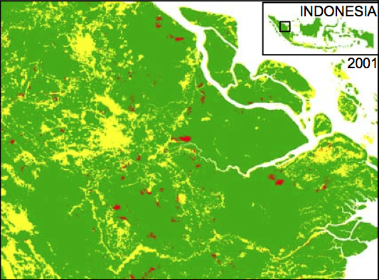
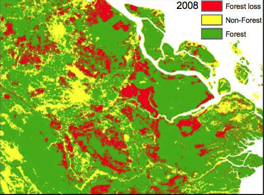
Satellite image example #1

Deforestation in Indonesia

(Burgess et al. 2012)

# of districts in a province $\uparrow$

$\Rightarrow$ Each district govt official engages in Cournot competition in selling (illegal) logging permits

$\Rightarrow$ Deforestation in the province $\uparrow$

Cannot rely on official stats of logging

$\Rightarrow$ Use satellite images

• Spatial resolution: 250m x 250m pixel
• Data: electromagnetic radiation strength in 36 bands of spectrum
• Develop algorithm to convert radiation patterns to forest coverage

Pixel-level data on deforestation

(Figure I of Burgess et al. 2012)

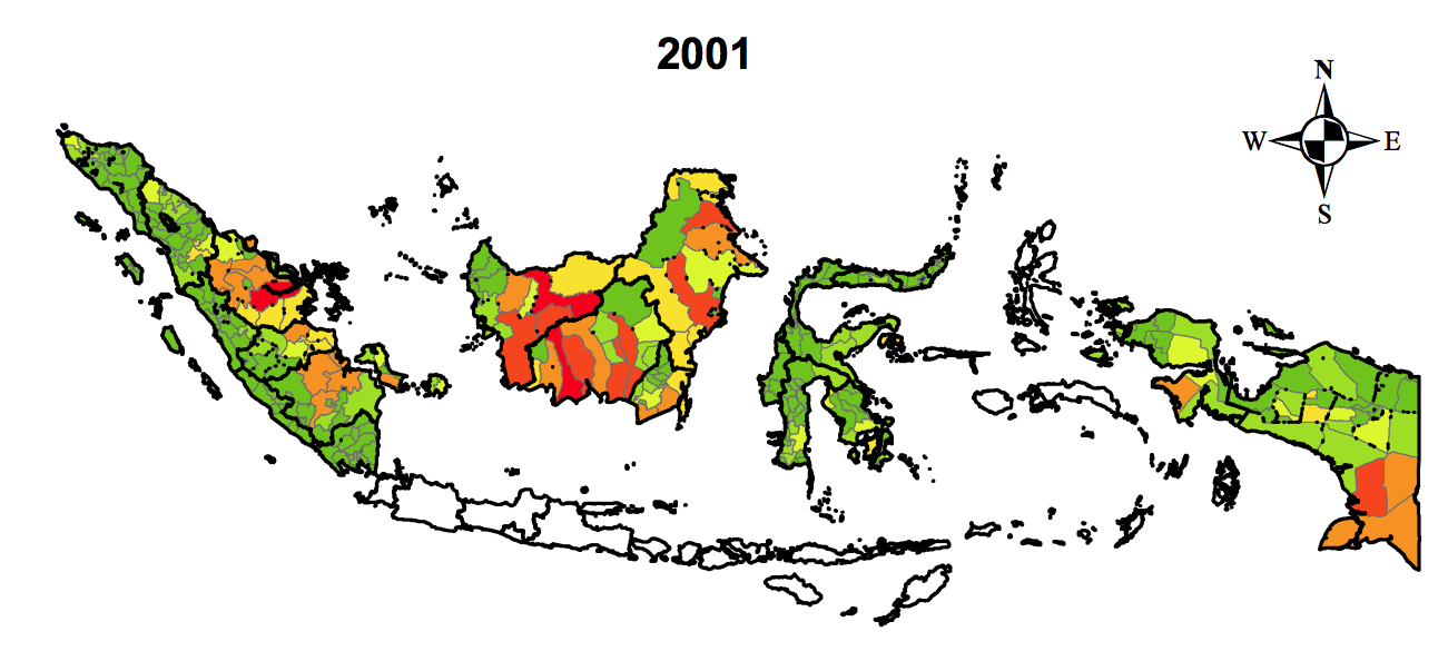
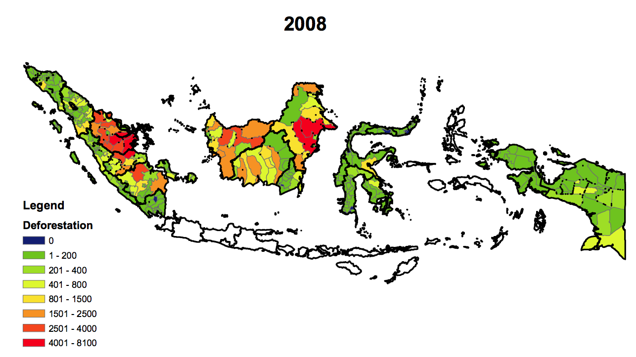
District-level data on deforestation

(Figure II of Burgess et al. 2012)

• We will learn how to aggregate satellite image data into administrative zones in Lecture 5

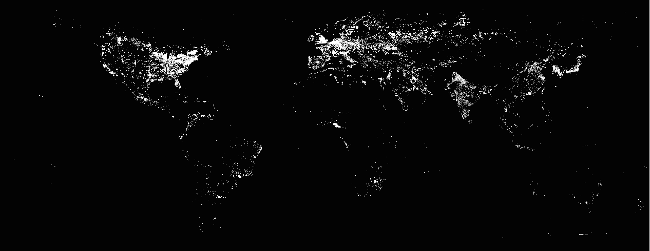
Satellite image example #2

Nighttime light 1992

(Source: Version 4 DMSP-OLS Nighttime Lights Time Series)

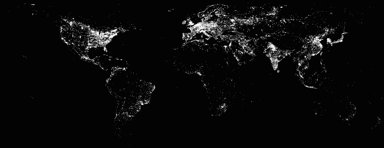
Satellite image example #2

Nighttime light 2013

(Source: Version 4 DMSP-OLS Nighttime Lights Time Series)

Nighttime light in top 5 econ journals

Henderson et al (2012): correlate with real GDP growth

Pinkovskiy & Sala-i-Martin (2016): accuracy of GDP versus household surveys

Michalopoulos & Papaioannou (2013, 2014), Alesina et al (2016): measure ethnicity-level development in Africa

Hodler & Raschky (2014): Presidents' home region brighter

Storeygard (2016): Impact of trade infrastructure in Africa

Henderson et al (2018): Geographic correlates of light

Campante and Yanagizawa-Drott (2018): Impact of air links

For more satellite image examples, see a survey by Donaldson and Storeygard (2016).

Old map example #1

Road building in Kenya

(Burgess et al. 2015)

Digitize Michelin maps for Kenya since 1961

Track road network expansion over time

• We will learn line length calculation in Lectures 6 and 7

See if the president's ethnic group gets more roads built than other groups

Digitizing old maps

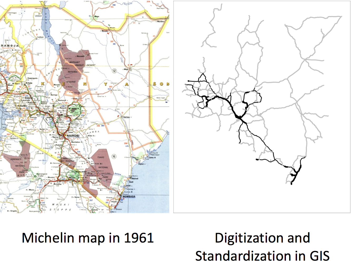
(source: Remi Jedwab's presentation slide)

Old map example #2

Ethnic homelands in Africa

Drawn by Murdock (1959)

Digitized by Nunn (2008), to match ethnicity-level data on slave trade with country-level data (Lecture 4)

Also used by Alsan (2015) (Lecture 2)

Other examples: Nunn & Wantchekon (2011), Michalopoulos & Papaioannou (2013, 2014, 2016), Alesina et al. (2016)

Ethnic homeland & country boudaries

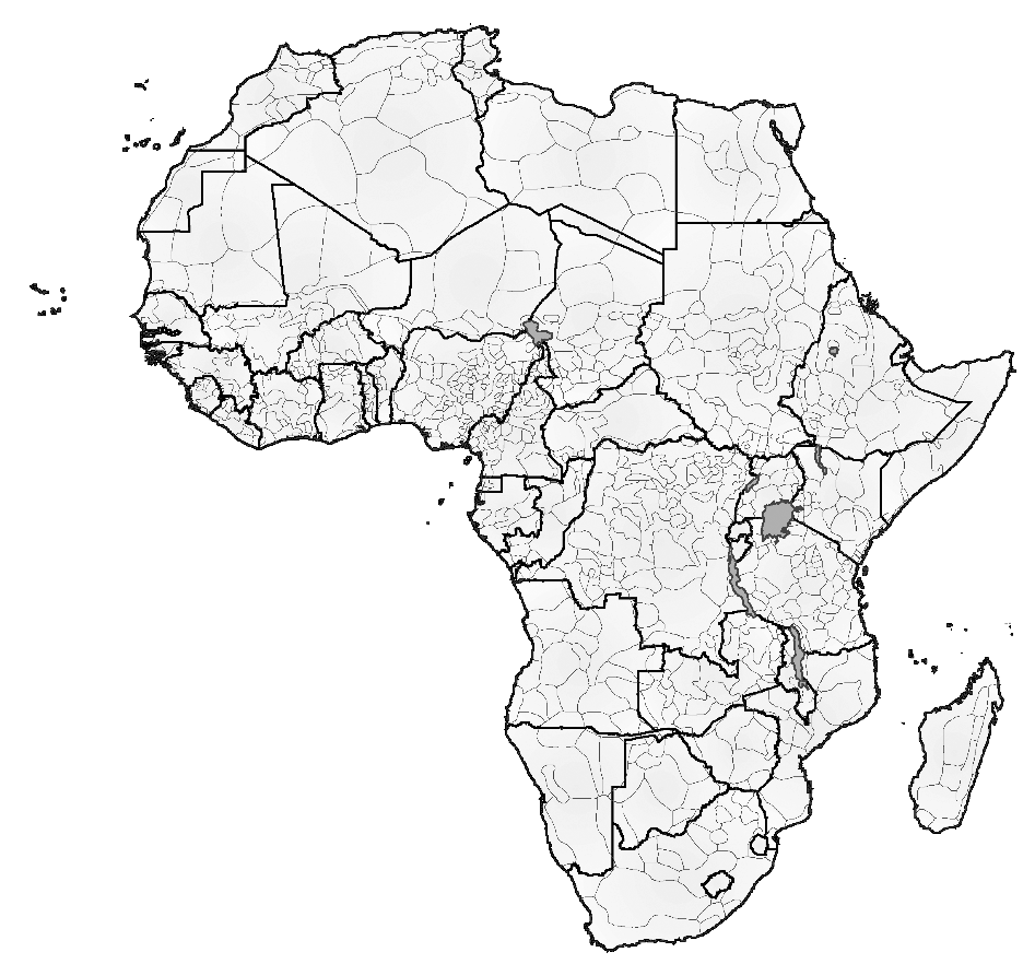
Figure II of Nunn (2008)

Practical advice

Satellite images: some are freely available but very costly (time & money) to process

• See "15 Free Satellite Imagery Data Sources" by GIS Geography
• An example of constructing data from satellite images: Measuering Yields from Space

Practical advice (cont.)

Old maps: digitizing is also time-consuming but feasible with patience in two steps:

1. Georeferencing
• Yale Map Collection (2009) (pp. 8-10)
• ArcGIS Help: Georeferencing a raster dataset
• How to georeference Meiji/Taisho-era maps of Japan (in Japanese)
2. Create vector data
• ArcGIS 10: Editing & Creating Your Own Shapefiles (Parts 3-4)

$\Rightarrow$ This course helps you use these datasets

3. GIS software

ArcGIS

• Python-friendly
• Buggy; tricky to create map images; Windows only

QGIS

• Free; easy to create map images; compatible with any OS
• Python-unfriendly
• Tutorials:
• www.qgistutorials.com for interactive use
• Lawhead (2017) for Python coding

$\Rightarrow$ For the ease of use of Python (for replication), we will learn ArcGIS

R

• Can be integrated into statistical analysis
• Tedious to browse data
• Textbook: Brunsdon & Comber (2015)
• Tutorial by Nick Eubank

Geopandas

• A Python library to work on spatial data
• Still under development (as of July 2018)

Purchasing ArcGIS

License fee (in case of Japan): 18,000 yen per year

• Price plan differs across countries.
• Contact ESRI of your country.

Make sure the package you buy include:

• ArcGIS Desktop Advanced
  • You cannot upgrade from Basic or Standard
• ArcGIS Spatial Analyst extension
  • For working on raster data (Lectures 5-8)
• ArcGIS 3D Analyst extension
  • If working on three-dimensional spatial data (Lecture 7)

Set up Windows 10 environment
for this course

1. Show file extensions (.shp etc) in File Explorer

• Click on the task bar at the bottom
• In the menu bar, click View
• Check "File name extensions" in the Show/hide pane

Set up Windows 10 environment
for this course (cont.)

2. Install 7-Zip for 64-bit Windows

• For uncompressing .tar files

Prepare for the rest of this lecture

1. Launch ArcMap 10 (it takes time)

2. Download the zipped dataset for lecture 1

3. Save it to Desktop (C:\\Users\\yourname\\Desktop)

• Don't save in the remote server, which slows down ArcGIS

4. Right-click it and choose 7-Zip > Extract to "Lecture1\"

• So the directory path will be: C:\\Users\\yourname\\Desktop\\Lecture1

Prepare for the rest of this lecture (cont.)

Browse the inside of the Lecture1 folder

I've created 4 folders:

• code/: files to edit datasets (e.g. Python scripts)
• input/: original data
• output/: final data to be used for analysis
• temporary/: other files created during process

It's a standard directory structure to organize files for empirical analysis

• cf. Chapter 4 of Gentzkow and Shapiro (2014)

Prepare for the rest of this lecture (cont.)

Now browse the input/ folder

5. Right-click all the .zip files and select 7-Zip > Extract Here

• 10m-rivers-lake-centerlines.zip
  • river polylines
• gadm36.zip
  • country/district polygons
• glds90ag.zip
  • population density raster

Leave F162008.v4.tar (nighttime light raster)
for the time being.

4. Polygon, polyline, point, and raster

Vector vs Raster

Spatial data comes in two different formats

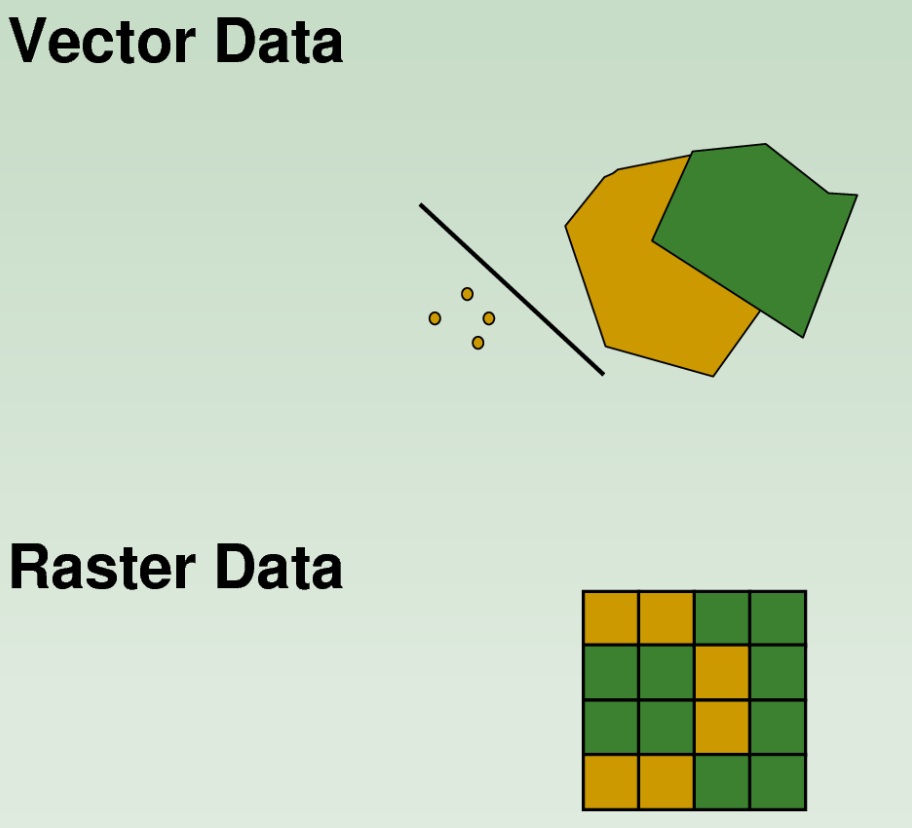
How to edit data differs a lot between them

We now learn how to browse spatial datasets in ArcGIS while learning these different formats of spatial data

Vector data

Each spatial unit in vector data is called a feature

Three types of a feature:

1. Polygon
2. Polyline
3. Point

A set of features of the same type: a feature class

File format: Shapefile (.shp)

Vector data #1

Polygon features

Represent geographic zones

• Countries (Lectures 4 & 5)
• Sub-national districts (Lecture 6)
• Ethnic homelands (Lectures 4 & 5)
• Lakes, Islands, etc.
• Grid cells (Lectures 2 & 5)

Exercise #1

Browse polygon features

Data to be read: GADM (widely used by economists)

• gadm36/gadm36_0.shp (countries)
• gadm36/gadm36_2.shp (subnational districts)

Drag these files in Catalog Window to Data Frame

• Don't see Catalog Window on the right?
• Don't see the data directory in Catalogue Window?
• See next slide...

Exercise #1 (cont.)

If you don't see Catalog Window...

$\Rightarrow$ Click Windows in the menu bar

If you don't see the data directory in Catalogue Window...

$\Rightarrow$ Right-click Folder Connections and click Connect To Folder...

Vector data #2

Polyline features

Represent networks / routes

• Roads (Lecture 7)
• Rivers (Lecture 6)
• Coastlines (Lecture 4)

Exercise #2

Browse polyline features

Data to be read: Natural Earth's Rivers and Lake Centerlines data (10m_rivers_lake_centerlines.shp)

Browse this data (cf. Exercise 1)

Uncheck the subnational boundary data in Table of Contents

• If you don't see Table of Contents, click Windows in the menu bar.

$\Rightarrow$ Now rivers are shown on national boundaries.

Exercise #2 (cont.)

Change the color of rivers to blue.

• Click the symbol (in this case, colored line) just below the data name in Table of Contents.
• Choose the preferred color.

If you read the river data first and then the national boundary data, the river data would be hidden below the national boundary data.

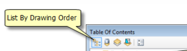
• In the Table of Contents window (the one on the left), drag the river data and drop it above the national boundary data.
• Then rivers will show up

If you cannot drag the data in the Table of Contents window, check if the List By Drawing Order icon is selected on top left.

Vector data #3

Point features

Represent point location

• Plots (Lecture 3)
• Schools
• Cities (Exercise #3 below)
• Centroid of polygon (Lecture 4)

Can easily be created from XY data

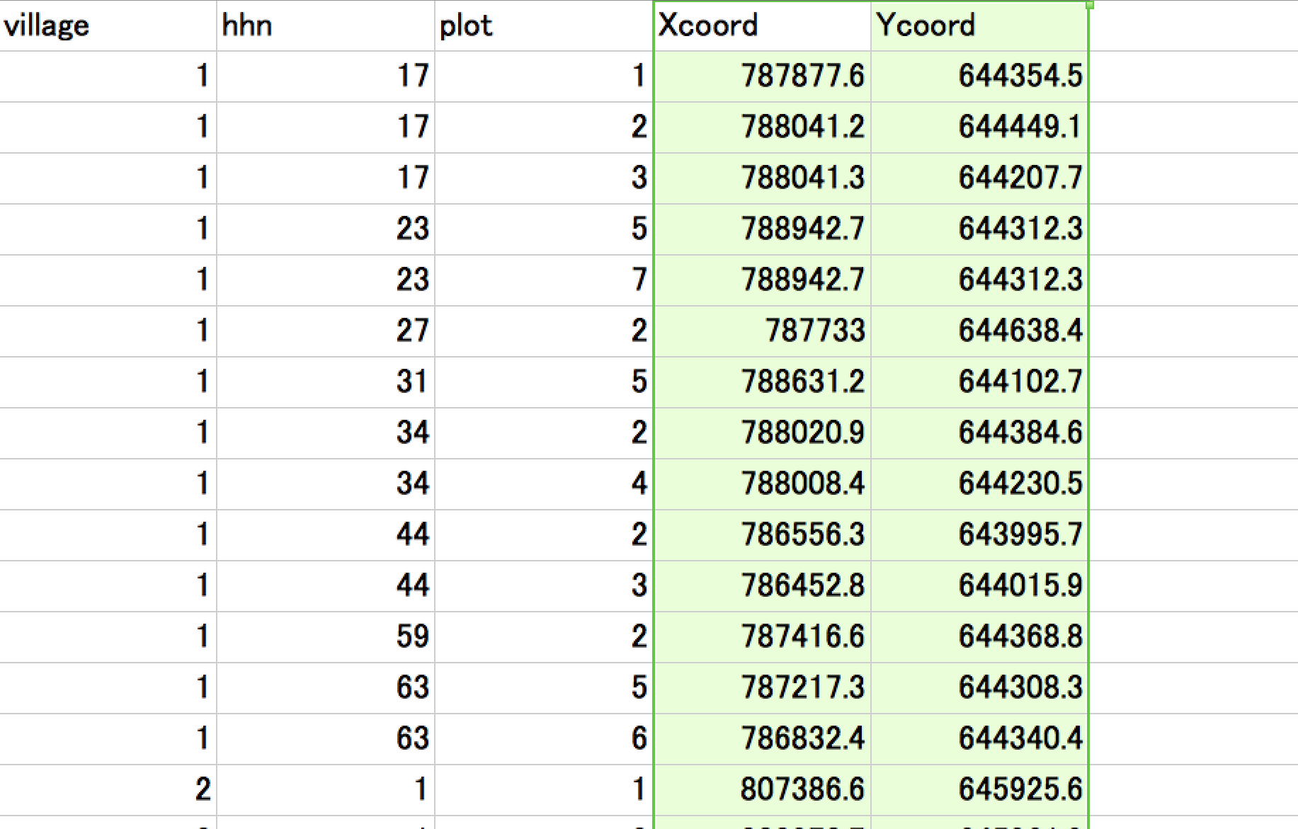
What is XY Data?

Each row: point feature

Column 1: longitude (x value)

Column 2: latitude (y value)

Other columns: attributes of point feature

• Location name
• Statistics
• Key (i.e. unique ID)
• Foreign keys (for merging with other data)

How to obtain longitude & latitude?

1. GPS receivers

If you conduct your own survey

• Measure DHS (2013) for the protocol to use GPS receivers
• Matt Decker (2011) for using a Garmin handheld unit to gather GPS data

How to obtain longitude & latitude? (cont.)

2. Online gazetteer

If location names are available, search at:

• Geonames
• To automate search, use Geonames Tools toolbox
• Global Gazetteer Version 2.3
• JRC Fuzzy Gazetteer

See Sundberg et al. (2010) for an example protocol

How to obtain longitude & latitude? (cont.)

3. Geocoding tools

If postal address is available, use:

• Google Geocoder
• CSV Address Matching Service for addresses in Japanese

To import XY data to ArcGIS

Data format: Comma-delimited text (csv) / Excel worksheet

• From Stata, use export delimited (Stata help)
• ArcGIS may round off longitude & latitude values
• Use the "format" command to avoid this (cf. Stata help)

Code example for 10 dicimal digits for longitude/latitude

						
format lon %15.10f
format lat %14.10f
export delimited lon lat using filename.csv, replace
						
					

To import XY data to ArcGIS (cont.)

To convert XY data into a point feature class, use:

• Make XY Event Layer
• Copy Features

These are the examples of geo-processing tools

Exercise #3

Convert XY data into point features

Data to be read: CEPII GeoDist Database (geo_cepii.xls)

Browse the data in Excel

• Which columns for longitude and latitude?

To implement geo-processing tools, we use Model Builder

• Model Builder helps us program in Python (Lecture 2).

Exercise #3 (cont.)

How to use Model Builder (1/3)

1. Click in the Standard Toolbar.
2. In Search Window, type the name of the geoprocessing tool and search.
• If you don't see Search Window, click Windows in the menu bar.
3. Drag the tool from Search Window to Model Builder
4. Double-click the tool to set inputs, outputs, options etc.

Exercise #3 (cont.)

Make XY Event Layer

XY Table: input/geo_cepii.xls/geo_cepii$

• For an Excel file, double click it to choose a worksheet inside

X Field: lon

Y Field: lat

Spatial Reference: WGS 1984

• Click & navigate to: "Geographic Coordinate Systems > World > WGS 1984"

Exercise #3 (cont.)

Help for geo-processing tools

If you don't know what to fill in on the geo-processing tool window:

1. Click Show Help >> on the bottom right
2. Click the input field you don't understand
3. The help document appears on the right column.

Exercise #3 (cont.)

Make XY Event Layer (cont.)

This tool creates a temporary layer

But the layer often doesn't properly work with other tools

We also want to save the point feature class in the disk

$\Rightarrow$ Always use the Copy Features tool to convert the layer into a shapefile data

Exercise #3 (cont.)

Copy Features

Input Features: the output from the Make XY Event Layer

• Use the drop-down menu, to specify the input that's already in the Model

Output Feature Class: ...\Desktop\Lecture1\output\cities.shp

• Always save newly created spatial data files in a folder different from the one for original input files

Ignore other options. Rarely used.

Exercise #3 (cont.)

Copy Features (cont.)

Also useful if you want to keep the original data intact

• Some geo-processing tools overwrite the input data...
• We will see such an example throughout the course

Exercise #3 (cont.)

How to use Model Builder (2/3)

To save the model:

1. Click the save icon
2. Navigate to the directory in which you will save the model (e.g. code/)
3. Click the toolbox icon (the red box at top-right)
4. Create a new toolbox (name it, say, lec1.tbx)
5. Click this toolbox
6. Type the file name for the model (e.g. exercise3)

A model can only be saved inside the toolbox.

Save frequently; ArcGIS often crashes.

Exercise #3 (cont.)

How to use Model Builder (3/3)

To edit an existing model:

1. Locate the model in Catalogue Window
• If you cannot see a new folder/file you just created, right-click the parent directory and "Refresh".
2. Right-click the model
3. Click Edit (NOT "Open")

Exercise #3 (cont.)

Now run the Model by clicking the triangle icon at top right

Browse the output point feature shapefile

Capital cities (and other major cities) around the world should appear as point features.

One more thing about vector data...

Attribute Table

Contains fields (i.e. variables) which can take a different value for each feature

To browse in ArcMap:

1. right-click the data in Table of Contents
2. click Open Attribute Table...

Recap: Vector vs Raster

Spatial data comes in two different formats

How to edit data differs a lot between them

Raster data

Divides the earth surface into many "square" cells (or pixels)

Each cell contains one value

Often created from satellite images

Examples:

• Elevation (Lecture 6)
• Suitability for agriculture (Lecture 5 & 8)
• Population density
• Forest coverage (this lecture)
• Nighttime light (this lecture)

Can create a new variable for vector data (Lecture 5, 6, 8)

Raster data (cont.)

Most file formats can be browsed in ArcMap

• TIFF (.tif)
• ESRI Grid (no extension)
• File name cannot be longer than 13 characters
• File structure is very complicated when browsed in Windows's File Explorer

$\Rightarrow$ I recommend using TIFF format

For the ASCII format (.asc), you need to convert it into TIFF (Excercise #5 below)

Exercise #4

Browse TIFF raster

Data to be read: DMSP-OLS nighttime light for year 2008

1. Extract F162008.v4.tar
• Right-click it and select 7-Zip > Extract Here
• This creates 3 pairs of .gz and .tfw files.
2. Extract .gz files to the same folder as .tfw files
• Right-click them and select 7-Zip > Extract Here
• The .tfw file allows ArcMap to read a TIFF image of the same file name as geo-referenced (see Greenberg 2003 for detail)

Exercise #4 (cont.)

3. In ArcMap, read F162008.v4b_web.stable_lights.avg_vis.tif
4. You'll be asked whether to "build pyramids"
• If yes, displaying raster data becomes faster

Exercise #5

Browse ASCII raster

Data to be read: population density in 1990 (input/glds90ag.asc)

• Source: Gridded Population of the World (version 3)

Use the ASCII to Raster tool

• Output raster: output/popden90.tif
  • Add ".tif" to save in the TIFF format
• Data type: FLOAT
• Population density can be decimal
• By default, it sets INTEGER, which will distort data

Exercise #5 (cont.)

When you read the converted population density raster, you'll get a pop-up alert message: "Unknown Spatial Reference"

We'll come back to this issue shortly.

Raster in Stata

Stata can read raster in the ASCII format, with ras2dta ado (Muller 2005)

Each cell becomes one row in Stata

To export raster as the ASCII format, use the Raster to ASCII tool in ArcGIS

One more raster format: NetCDF

NetCDF files: Widely used for time-series raster data

• Example: Landcover change over 200 years

To browse NetCDF data at each point in time, use:

• Make NetCDF Raster Layer
• and then, Copy Raster

5. Coordinate systems

What is a coordinate system?

Earth is a sphere (approximately)

Various ways to two-dimensionally represent the earth surface

Each way corresponds to a coordinate system

aka. spatial reference / map projection

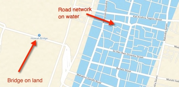
Why important?

To calculate distance and surface area properly

To merge different spatial datasets accurately

cf. Apple Map did this wrong when it was launched in 2012

Two types of coordinate systems

1. Geographic
2. Projected

See Eubank (2018) for more exact explanation on the difference

Geographic Coordinate Systems

Each location is coded by degrees

e.g. Osaka: 34.6937° North, 135.5022° East

Not suitable for calculating surface area

• 1° in lat: 110.6km at equator / 111.7km at poles
• 1° in lon: 111.3km at equator / 55.8km at 60° N/S

Geographic Coordinate Systems (cont.)

But useful for calculating distance between two locations

• Use great-circle distance formula (Lecture 4)
• Can be obtained by Stata ado globdist

WGS 1984: most popular

Projected Coordinate Systems

Earth surface is projected by the "light" from the center of the earth on cylinder:

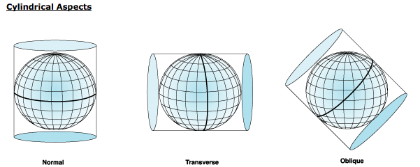
Projected Coordinate Systems

Earth surface is projected by the "light" from the center of the earth on cone:

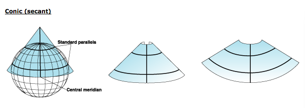
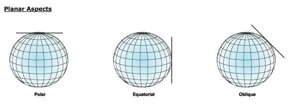
Projected Coordinate Systems

Earth surface is projected by the "light" from the center of the earth on plane:

Projected Coordinate Systems (cont.)

Each location: coded in meters from a certain origin

Which coordinate system to use?

WGS 1984

• Distance between two locations (Lecture 4)

UTM

• Distance / surface area in small regions (Lecture 3)
• Length of polyline features (Lecture 6)

Any equal area projections

• Surface area in large regions (Lecture 4)

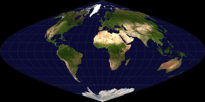
Equal area projections

Differ just in how the world is shown

Sinusoidal Projection

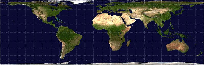
Equal area projections

Differ just in how the world is shown

Lambert Cylindrical Equal Area projection

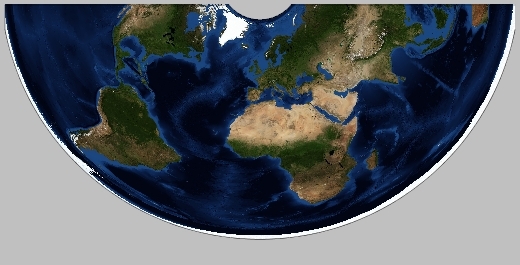
Equal area projections

Differ just in how the world is shown

Alberts Conic Equal Area projection

If you want to know more:

Map Projections: A Working Manual, by John P. Snyder (U.S. Geological Survey, 1987) (Downloadable for free)

Check the coordinate system in ArcMap

1. Right-click the data in Table of Contents
2. Click "Properties..."
3. Click the "Source" tab
4. Check "Coordinate System" (scroll down, if not shown)

Geo-processing tools to assign a coordinate system

Project: for vector data

Project Raster: for raster data (Lecture 7)

Define Projection: if undefined (for both vector & raster)

• Remember the alert message "Spatial reference is undefined" in Exercise #5?
• It means the coordinate system is not assigned

Coverage toolbox

Don't use Project (Coverage) or Define Projection (Coverage)

• Those tools with "(Coverage)" in the name are meant for vector data in the old format (called coverage)
• Many of the tools we will learn in this course have their counterpart with "(Coverage)" in the name
• Just ignore those tools.

Exercise #6

Assign the projection to Population raster

Spatial data usually comes with a meta data that specify the coordinate system used when the data is created

GPW's meta data says it's WGS 1984

Exercise #6 (cont.)

Use Define Projection to assign WGS 1984 (cf. Exercise #3)

• Input Dataset or Feature Class: popden90.tif
• The output from ASCII to Raster
• Coordinate System: "Geographic Coordinate Systems > World > WGS 1984"

Note that this geo-processing tool overwrites the input file.

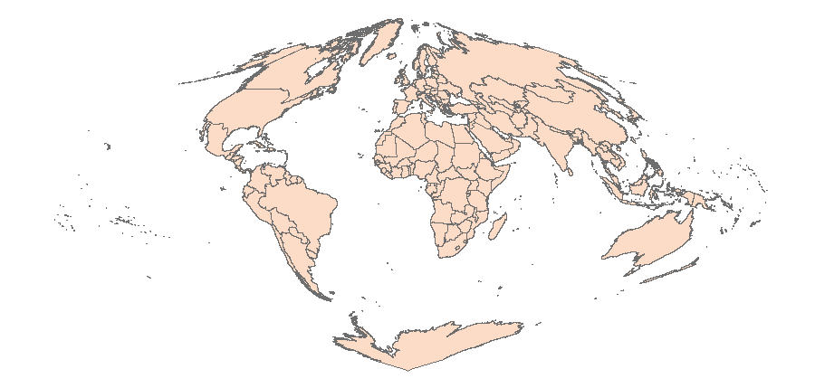
Exercise #7

Project to Sinusoidal

Suppose we are interested in calculating the surface area of districts around the world

Sinusoidal projection allows you to calculate surface area properly

Use the Project tool to change the coordinate system from WGS 1984

Sinusoidal projection is found at:

Projected Coordinate Systems > World > Sinusoidal(world)

Exercise #7 (cont.)

Browse the output. Does it look like this?

Browse data in a different projection

You cannot overlay data with different coordinate systems

ArcMap displays data in the coordinate system of the data read first

To browse a data with a different coordinate system, open a new map document

What is map document?

Saves the way you overlay / color-code / symbolize different spatial datasets

File extension: .mxd

DOES NOT contain spatial data. It just has links to them

Set the relative path to refer to each data

Exercise #8

Save a Map document

1. Set relative paths as the default (only needed to do once)
• In the menu bar, click Customize > ArcMap Options
• Click the General tab
• Check "Make relative paths the defaults for new map documents"
2. Click the save icon in the Standard Toolbar
• This DOES NOT save the data
3. Choose the location in which you save the map document
• e.g. the code/ folder

Exercise #8 (cont.)

Browse a data in different projection

1. Open a new Map Document
2. Drag the GADM data in Sinusoidal projection (the output from Exercise #7) from Catalogue Window

Exercise #8 (cont.)

Now you should see something like this: