Causal Inference with Spatial Data
(ArcGIS 10 for Economics Research)
Lecture 3
Buffer
Masayuki Kudamatsu
19 October, 2018
Press SPACE to proceed.
To go back to the previous slide, press SHIFT+SPACE.
Buffer tool in ArcGIS
Create a polygon of an input feature's neighborhood
|

|
|
Point
|
Polyline | Polygon |
Buffer tool in ArcGIS (cont.)
Buffer + Spatial Join $\Rightarrow$
$\Rightarrow$ Identify neighbors for each point
This is useful for economics research for (at least) 3 reasons
Buffer tool for economics research
1. Generate a treatment variable
 (image source)
Estimate the impact of shale gas wells on house prices in their neighborhood
- Houses within 2km of wells: treated
Buffer tool for economics research (cont.)
2. Estimate spillover effects of treatment
 (Image source)
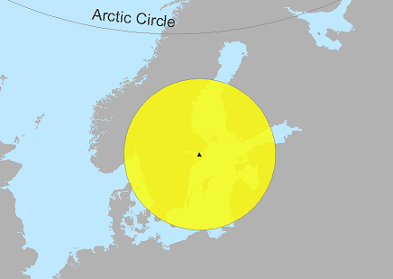
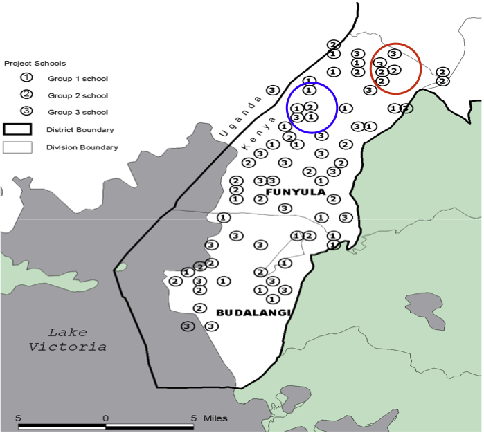
RCT on deworming school children
# of treated schools within 6km can be identified by Buffer tool
Buffer tool for economics research (cont.)
3. Mitigate omitted variable bias in peer effect estimation
Today's road map
1. Conley & Udry (2010)
2. UTM projections
3. Replicate Conley & Udry (2010)
4. Set relative file paths in Python
1. Conley & Udry (2010)
Research Question
Do farmers learn from their peers regarding input use (fertilizer) for new technology (pineapple)?
Important?
- If yes, only a few farmers need to be subsidized for universal adoption
Original?
- Overcome econometric issues of identifying the impact of peer behavior
Feasible?
- Very detailed data collection, including plot locations
Data
Panel household surveys (every 6 week in 1996-98) in 3 villages of southern Ghana
- Amount of fertilizer used
- Whom they turn for advice on farming
- Plot location, collected by GPS receiver (cf. Lecture 1)
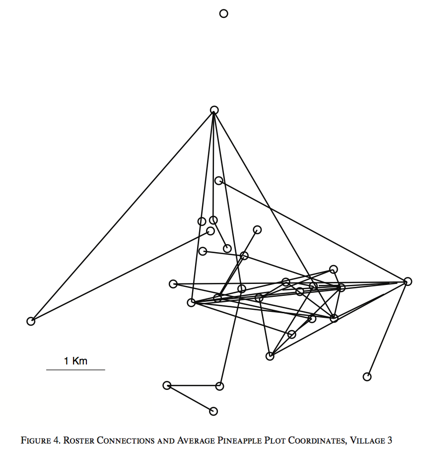
Data on social networks and plot locations
Empirical specification
Define the treatment variable for farmer $i$ in period $t$ as:
\begin{align*} M_{i,t} \equiv \frac{GoodNews(x_{j,s-5}) \times (x_{j,s-5} - x_{i,t_p})}{Experience_{it}} \end{align*}
| $x_{i,t_p}$ | $i$'s use of fertilizer at period $t_p$ (i.e. previous planting) |
| $x_{j,s-5}$ | farmer $j$ ($i$'s friend)'s use of fertilizer at period $s-5$, where $s \in [t_p,t]$ |
| $GoodNews(x_{j,s-5})$ | Indicator of higher-than-expected profit (fn.22) from using $x_{j,s-5}$ |
| $Experience_{it}$ | $i$'s experience of planting pineapple |
Empirical specification (cont.)
Then estimate: \begin{align*} \Delta x_{i,t} = \beta_1 M_{i,t} + \beta_2 \Gamma_{i,t} + \boldsymbol{z}'_{i,t}\boldsymbol{\beta_3} + \nu_{it} \end{align*}
| $\Delta x_{i,t}$ | Changes in fertilizer use since $t_p$ |
| $\boldsymbol{z}'_{i,t}$ | Other controls |
| $\Gamma_{i,t}$ | Growing condition for $i$'s plot at period $t$ |
\begin{align*} \Gamma_{i,t} \equiv x_{i,t}^{close} - x_{i,t_p} \end{align*} where $x_{i,t}^{close}$ averages fertilizer use over plots within 1km from $i$ during previous 3 periods
$\Rightarrow$ $\Gamma_{i,t}$ controls for common shocks to $i$ and $i$'s friends
We will learn how to identify plots within 1km from $i$
Source of identification: Friends outside 1km radius
(Figure 4 of Conley & Udery 2010)
Empirical specification (cont.)
\begin{align*} \Delta x_{i,t} = \beta_1 M_{i,t} + \beta_2 \Gamma_{i,t} + \boldsymbol{z}'_{i,t}\boldsymbol{\beta_3} + \nu_{it} \end{align*}
Standard errors: calculated by Conley (1999)
Which is now the standard procedure for cross-sectional regression with spatial data
Conley (1999) standard error
Let $\mathbf{b}$ denote a vector of coefficients estimated by OLS
Variance of OLS estimator: \begin{align*} V(\mathbf{b}) = (\mathbf{X}'\mathbf{X})^{-1}\mathbf{X}'E(\boldsymbol{\varepsilon}\boldsymbol{\varepsilon}')\mathbf{X}(\mathbf{X}'\mathbf{X})^{-1} \end{align*}
| $\mathbf{X}$ | $n$ (# of obs.) by $k$ (# of regressors) data matrix |
| $\boldsymbol{\varepsilon}$ | $n$-dimensional vector of the error term |
Conley (1999) standard error (cont.)
Let $\rho_{ij}$ denote $ij$-th element of $E(\boldsymbol{\varepsilon}\boldsymbol{\varepsilon}')$
- Error term's correlation between $i$ & $j$
Conley (1999) imposes $\rho_{ij} = K_{ij}\hat{\varepsilon}_i\hat{\varepsilon}_j$ where
\begin{align*} K_{ij} \equiv \left\{ \begin{array}{cl} (1-\frac{x_{ij}}{\bar{x}})(1-\frac{y_{ij}}{\bar{y}}) & \mbox{if $x_{ij}<\bar{x}$ & $y_{ij} < \bar{y}$} \\ 0 & \mbox{otherwise} \end{array} \right. \end{align*}
| $x_{ij}, y_{ij}$ | Distance between $i$ & $j$ in x,y dimension |
| $\bar{x},\bar{y}$ | Cut-off value chosen by researcher (1.5km in Conley-Udry 2010) |
| $\hat{\varepsilon}_i$ | OLS residual for $i$ |
Conley (1999) standard error (cont.)
Tim Conley's website offers Stata ado files for implementing Conley (1999) for OLS, GMM, and Logit
In this ado program, $x_{ij},y_{ij}$ is calculated from the coordinates of $i$ and $j$
Make sure to use a projected coordinate system (cf. Lecture 1)
Conley (1999) standard error (cont.)
Conley's (1999) Stata ado cannot be used for panel regressions...
Hsiang (2010) extends it to a panel data, with a new Stata ado
- Non-parametrically accounts for serial correlation
- Allows you to use uniform kernel ($K_{ij}=1$ within cutoff)
- Compatible with geographic coordinate systems (cf. Lecture 1)
Main results
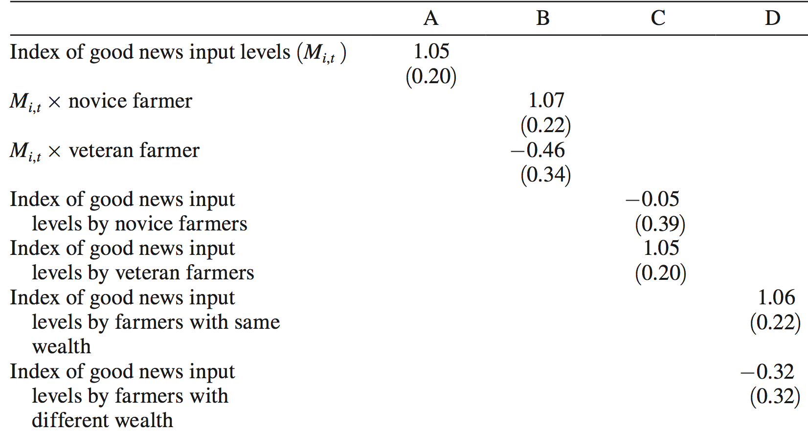
(Table 5 of Conley & Udry 2010)
Placebo tests with labor use
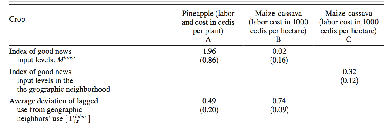
(Table 7 of Conley & Udry 2010)
Prepare for the rest of this lecture
1. Launch ArcMap 10 (it takes time)
2. Download the zipped dataset for lecture 3
3. Save it to Desktop (C:\\Users\\yourname\\Desktop)
- Don't save in the remote server, which slows down ArcGIS
4. Right-click it and choose 7-Zip > Extract to "Lecture3\"
-
So the directory path will be:
C:\\Users\\yourname\\Desktop\\Lecture3
Prepare for the rest of this lecture (cont.)
Now in ArcMap's Catalogue Window:
5. Establish connection to data folder
- Right-click Folder Connections
- Select Connect to Folder
- Choose Desktop > Lecture3
6. Prepare the Model Builder
- Create a Model
-
Save it as "
code/models.tbx/lecture3
2. UTM projections
Coordinate systems for Buffer tool
Buffer tool requires distance calculation
How to calculate distance depends on which coordinate system is used, geographic or projected
This lecture uses UTM, a projected coordinate system
- In Lecture 4, we learn distance calculation with geographic coordinate systems
So let's learn about UTM.
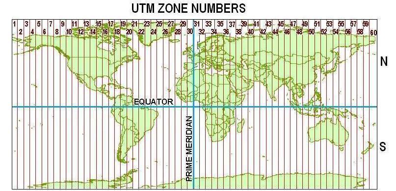
What is UTM?
Stands for Universal Transverse Mercator
Project earth surface onto the cylinder that is tangent on standard meridian

Father away from standard meridian, more distortion
What is UTM? (cont.)
To minimize distortion:
1. Divide Earth into 60 zones (6° wide in longitude)
What is UTM? (cont.)
2. For each zone, set standard meridian in the middle
3. Scale down distance along standard meridian by 0.9996
- This number is called scale factor
- 0.9996 minimizes overall distortion w/i the 6°-wide zone
UTM in ArcGIS
120 UTM projections available
- Northern- and southern hemispheres for each of 60 Zones
Pick the appropriate zone for your study area
- In Conley and Udry (2010), it should be UTM 30 North.
- In Lecture 6, we use several UTM zones covering India to calculate river length
3. Replicate Conley & Udry (2010)
Data we want to construct
Conley and Udry (2010) construct the growing condition variable as
\begin{align*} \Gamma_{it} \equiv x_{it}^{close} - x_{it_p} \end{align*}
| $x_{it}^{close}$ | Average of $x_{ks}$ |
| $k$ | Plots within 1km from plot $i$ |
| $s$ | $\in \{t-3, t-2, t-1, t \}$ |
Data we want to construct
Conley and Udry (2010) construct the growing condition variable as
\begin{align*} \Gamma_{it} \equiv x_{it}^{close} - x_{it_p} \end{align*}
| $x_{it}^{close}$ | Average of $x_{ks}$ |
| $k$ | Plots within 1km from plot $i$ |
| $s$ | $\in \{t-3, t-2, t-1, t \}$ |
Input data we have
Browse the plot location data (Lecture3/input/udry2010.csv) with Notepad
- This file was created from the replication data file for Conley and Udry (2010)
- If you do a survey with GPS receiver, you will have a XY data like this one
village hh plot: plot identifier
Xcoord Ycoord: plot coordinate in meters
Exercise #1
Create plot point features
Which geo-processing tool(s) do we need to use? (answer)
Exercise #1: Step 1
Make XY Event Layer
XY Table: ...\Lecture3\input\udry2010.csv
X Field: Xcoord
Y Field: Ycoord
Spatial Reference: WGS_1984_UTM_Zone_30N
-
Click

- Navigate to Projected Coordinate Systems > UTM > WGS 1984 > Northern Hemisphere
Leave the other options as they are.
Exercise #1: Step 2
Copy Features
Input Features: udry2010_Layer
- The output from Make XY Event Layer
Output Feature Class: ...\Lecture3\temporary\plots.shp
Exercise #1 (cont.)
Now save and run the Model.
Browse the output. You should see something like this:

Browse the attritube table, too. Is everything as expected?
Exercise #2
Match each plot with its neighbors
Geo-processing tools to be used for this exercise:
1. Buffer (Analysis)
- Create 1km radius circle polygon around each plot
2. Spatial Join
- Match each circle polygon w/ plots within
Exercise #2: Step 1
Buffer (Analysis)
Input Features: plots.shp
- The output from Copy Features (in Exercise 1)
Output Feature Class: ...\Lecture3\temporary\buffer1km.shp
Distance: Linear unit / 1 / Kilometers
- Check "Field" if buffer size differs across features
Dissolve Type: NONE
- Select ALL or LIST to make overlapping buffers as one polygon
Exercise #2: Step 1 (cont.)
Now save and run the Model.
Browse the output. You should see something like this:
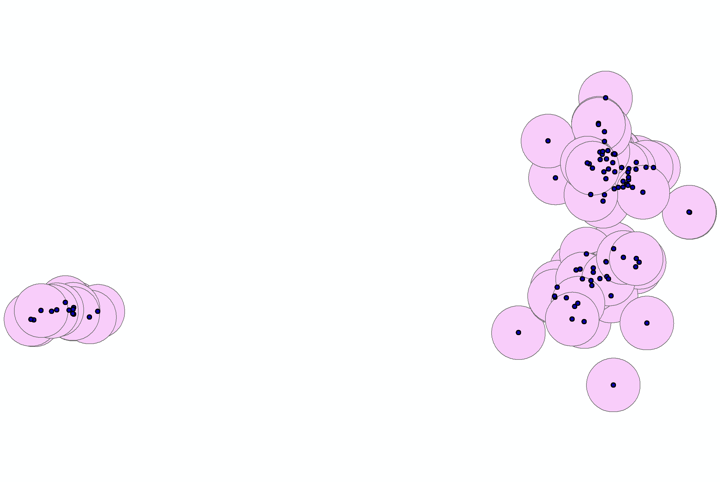
Browse the attribute table of the output. Notice that field names are all the same as plots.shp
Exercise #2: Step 2
Spatial Join
Target Feature Class: buffer1km.shp
- The output from Buffer
Join Features: plots.shp
- The output from Copy Features (in Exercise 1)
Output Feature Class: ...\Lecture3\temporary\plot_neighbors.shp
Spatial Join (cont.)
Join Operation: JOIN_ONE_TO_MANY
- To match all plots within 1km radius
Check "Keep All Target Features"
- We want to know which plots have no neighbor
Field Map of Join Features: see next slide
Match Option: INTERSECT
Field Map for Spatial Join
Supposed to allow you to control which fields to be kept
When exported as a Python script, it tends to misbehave...
Best solution:
- Include every field when running the model
- Delete every field before exporting a Python script
- If Field Map is unspecified, it will (paradoxically) keep all the fields
$\Rightarrow$ For now, keep every field
Field Map for Spatial Join (cont.)
When target and join features have the same set of fields
$\Rightarrow$ Fields from join features are suffixed with "_1"
That's why you see village_1, hhn_1, plot_1, etc.
Exercise #2: Step 2 (cont.)
Now save and run the Model.
Browse the output and its attribute table
- You may find that none of the join feature fields is included
- This seems to be a Model Builder's bug
- You can fix this in Python later
Exercise #3
Export attribute table
Which geo-processing tool(s) do we use? (cf. Lec 2 Ex 3)
Exercise #3 (cont.)
If you prefer Excel...
Table To Excel
-
Input Table:
plot_neighbors.shp -
Output Excel File:
...\Lecture3\output\plot_neighbors.xls
Exercise #3 (cont.)
If you prefer ASCII...
Export Feature Attribute to ASCII
Input Feature Class: plot_neighbors.shp
Value Field: see next slide
Delimiter: SPACE
- Not COMMA, to avoid confusing with decimal mark
Output ASCII File: ...\Lecture3\output\plot_neighbors.txt
Check "Add Field Name to Output"
Exercise #3 (cont.)
Value Fields
From target features: village, hhn, plot, xcoord, ycoord
- We need xcoord and ycoord for calculating Conley (1999) standard errors
From join features: village_1, hhn_1, plot_1
"Model" model for Lecture 3
Look at models.tbx/exercises1-3 in the folder solutions4exercises/
Exercise #4
Write a Python script
Delete every field in Spatial Join's Field Map (Why)
Export the model as a Python script (cf. Lec 2 Ex 4)
Exercise #4
Write a Python script (cont.)
The last three commands should look like this:
# Process: Spatial Join
arcpy.SpatialJoin_analysis(buffer1km_shp, plots_shp, plot_neighbors_shp, "JOIN_ONE_TO_MANY", "KEEP_ALL", "", "INTERSECT", "", "")

# Process: Table To Excel
arcpy.TableToExcel_conversion(plot_neighbors_shp, plot_neighbors_xls, "NAME", "CODE")

# Process: Export Feature Attribute to ASCII
arcpy.ExportXYv_stats(plot_neighbors_shp, "village;hhn;plot;village_1;hhn_1;plot_1", "SPACE", plot_neighbors_txt, "ADD_FIELD_NAMES")
The highlighted in yellow is where you specify fields to keep
- Each field name is delimited with semi-colon (;)
Exercise #4 (cont.)
Then edit the script by using the template (Lecture3\code\template4L3.py)
- Try-Except statement (Lec 2 Ex 6)
- String variables for file names (Lec 2 Ex 7)
- Print commands (Lec 2 Ex 8)
- Close any outputs in ArcMap or Excel (Why?)
- Run the script
Exercise #4 (cont.)
Browse the output
Select one plot neighborhood polygon
Browse the attribute table
Count # of matched plots for this selected plot
See if the same # of plot points are located within the polygon
4. Set relative file paths in Python
Problems with absolute file path
Currently we set an absolute file path
arcpy.env.workspace = "C:\\Users\\your_username\\Desktop\\Lecture3"
This code will break when
- Someone else runs the code in their computer
- You buy a new computer
- You reorganize the directory structure
Super-tedious to change this line of code if
- There are many Python scripts
- You're collaborating with someone else
Solution: use relative file path
import os
work_dir = os.path.dirname(os.path.realpath(__file__))
os.chdir(work_dir)
These 3 lines of Python code sets the folder where the current script is saved (e.g. .../Lecture3/code/)
as the working directory
We can then set its parent directory (e.g. Lecture3/) as the working directory for ArcGIS by
arcpy.env.workspace = "../"
cf. In Stata, cd .. moves up one directory
Now the code will run successfully as long as you
move the entire project directory (e.g. Lecture3/)
to another computer
Exercise #5
Set the relative file path
1. Open code/template4exercise5.py
-
This file contains the three lines of code:
import os
work_dir = os.path.dirname(os.path.realpath(__file__))
os.chdir(work_dir)
2. Copy and paste the whole Exercise 4 code below these three lines
3. Replace the line for arcpy.env.workspace with
arcpy.env.workspace = "../"
Exercise #5 (cont.)
4. Delete all the files in temporary/ and output/
5. Run the code. Check if every file is created in the expected folders
6. Now delete all the temporary and output files again.
7. Move the entire Lecture3/ folder to somewhere else (say, Documents/)
8. Open the Python script in this new location, and run it.
9. Also run the Exercise 4 script and see how it returns an error
What we've learned on ArcGIS
- Match each point w/ its neighboring points (i.e. w/i a radius of certain distance)
Do you remember which geo-processing tools you used for each of these tasks?